
Random Quote Board
Demodulating NOAA APT Signals
I'm writing this article because I think it's fun. The US' National Oceanic and Atmospheric Administration (NOAA) operates a fleet of satellites to look at earth's weather. Several of those transmit relatively low frequency (137 - 138 MHz) signals that contain low resolution visible and infrared imagery (roughly 4 km) of earth. These are the Automatic Picture Transmission (APT) signals. These signals are all-analog, as well. This makes them a perfect target if you want to try out using Gnu Radio Companion (GRC) on something a little different.
If You're Just Looking for An Image
There are two straightforward methods if you just want an image.
- The Wxtoimg program can give you beautiful images pretty-much automagically. It will (if I understand it correctly) already control your RTL-SDR and audio card to process the data and give you beautiful, synchronized images.
- You can frequency demodulate the NOAA APT signal, create a WAV file, then use Martin Bernardi's "NOAA APT Decoder" program to give you beautiful images.
Background
NASA launched the first weather satellite, TIROS (Television Infrared Observation Satellite) into space on April 1st, 1960. It was the greatest April Fool's non-joke ever. Since then, new satellites have been launched to both augment or replace those that reached end-of-life. TIROS-8, launched on 23 December 1963, added a continuous, analog video signal called "Automatic Picture Transmission" or "APT". Currently, NOAA operates a set of polar orbiting satellites that transmit both high resolution and low resolution (APT) weather imagery. There are currently (as of December 2020) three operational satellites that provide APT transmissions. These are NOAA-15, NOAA-18, and NOAA-19. These signals are meant to provide access to weather data for those with minimal access to equipment and budgets. Their set-up means that, aside from the computer required (which is now lessened to a Raspberry Pi, if you're so inclined), you can receive such signals for less than $50 in parts (SDR and antenna).
The APT Signal
The Automatic Picture Transmission (APT) signal is an analog signal used to transmit low resolution imagery. Here's the shortened version. The imagery is bandwidth limited to 2080 Hz and amplitude modulated (AM) onto a 2400 Hz carrier with bandwidth of 4160 Hz. That signal is then modulated onto a 137+ MHz signal using frequency modulation (FM) with a 17 kHz deviation.
If you're interested in reading more of the technical details of the APT signal, your two, primary documents are:
- User's Guide for Building and Operating Environmental Satellite Receiving Stations.
- NOAA KLM User's Guide, which strangely starts with a table of contents and has no cover page. Not even a TPS coversheet. Need to speak to the manager about that.
Also, SIGIDWiki does a pretty good job of covering the specifics, including going into details of the telemetry information.
Quick Setup
Here's my setup for the signals and images in this post.
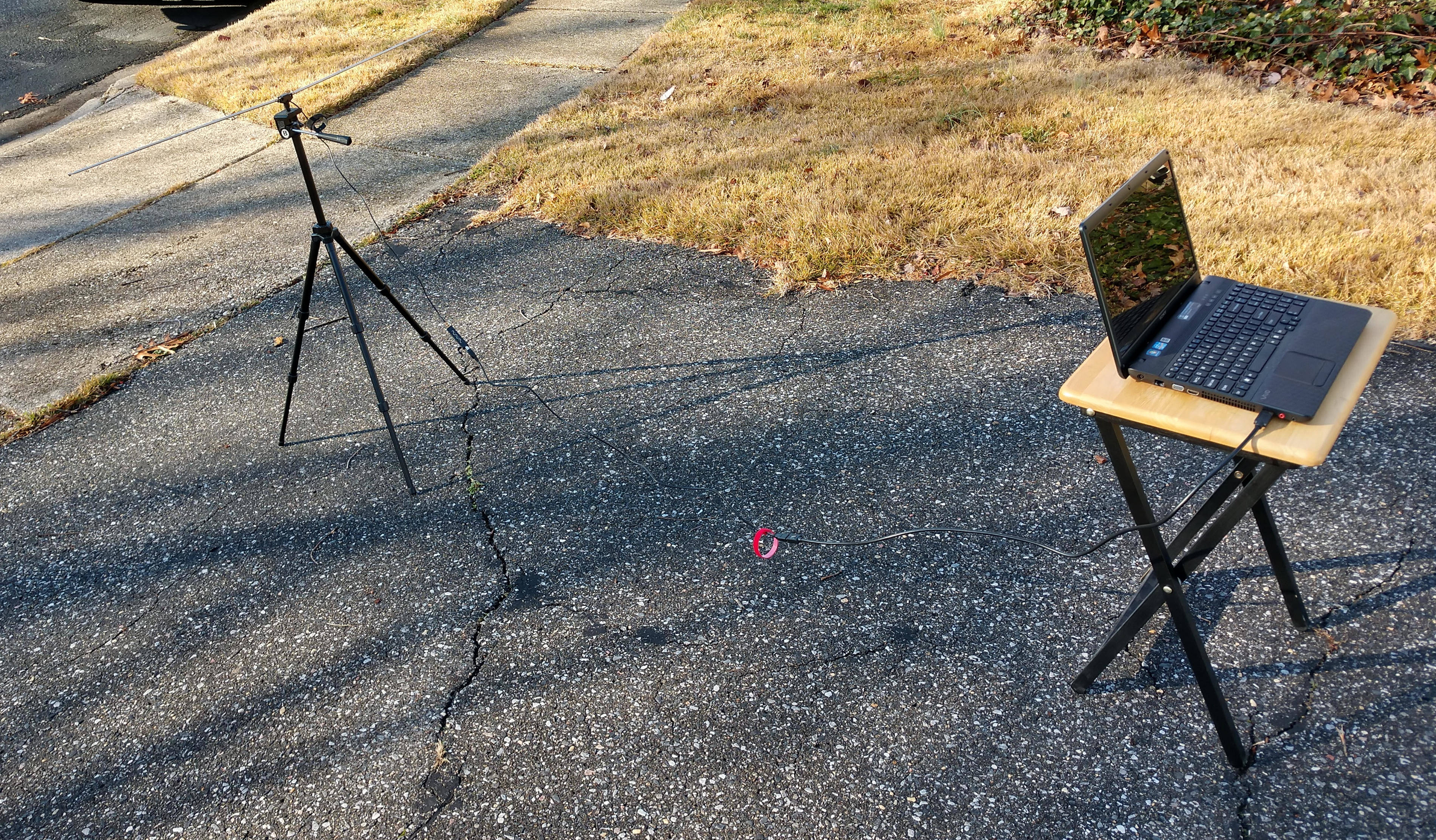
The rest of this post will go into details of the NOAA APT signals themselves, the antenna and the GRC flowgraph.
Finding the Satellite
Before you can demodulate an APT signal, you have to receive such a signal. There are three satellites constantly transmitting. The problem is those satellites are constantly moving. How to find out when they'll be one near you? Here are my recommended steps:
- Determine your latitude and longitude. You need to know where you are, specifically your latitude and longitude. The easy way is to use Google Earth. Just zoom in on wherever you want to collect from, place your cursor over the point of interest, then write down your latitude and longitude in "decimal" format. This means that you don't want "degrees / minutes / seconds", you want "degrees and decimal fraction of degrees". If you go into "Settings" of Google Earth, it will let you set the latitude / longitude readout to "Decimal". You could also use an app on your smartphone. I use GPS Status & Toolbox.
- Determine your time zone difference between you and Greenwich. For example, I'm on the East Coast of the US. I'm currently five hours behind (UTC-5) London (Greenwich) time.
- Go to the Amateur Satellite Online Satellite Pass Predictions page. Enter the satellite you want to see (NOAA-15, NOAA-18, NOAA-19), your latitude and longitude from Step #1 above, and press the "Predict" button. You'll be provided a table showing a bunch of data. Here's what that data means:
- Date: The date, in UTC (universal coordinated time, aka "Zulu" or "Greenwich" time).
- AOS: "Arrival of Signal", meaning the earliest you're likely to see the signal.
- Duration: The amount of time that you're likely to see the signal as the satellite passes over.
- AOS Azimuth: The azimuth of the satellite at the time that it first appears on the horizon.
- Maximum Elevation: The elevation at the point when the satellite is highest in the sky.
- Max El Azimuth: The azimuth of the satellite at the time that it is at its highest point in the sky.
- LOS Azimuth: The azimuth of the satellite at the time that it drops back below the horizon.
- LOS UTC: The time at which the satellite will drop below the horizon.
- Note the "Maximum Elevation". If you're in the suburbs, I recommend that you look for a time when this value is 30 degrees or greater.
- Note the "AOS UTC" of whichever pass you want to collect. That's the time when the signal will start to appear. Now, change that time UTC time to your local time. For example, if the UTC time is 1434, and I'm five hours behind, then the AOS local time will be 0934 (2:34 pm minus five hours). This means that some times might move the date back a day. For example, if I collect a signal that is 0134 UTC, this equates to 2034 local time of the date before.
- Note the "AOS Azimuth" and the "LOS Azimuth". If the AOS is roughly north and the LOS roughly south, then the satellite is moving from north to south. If the AOS is roughly south and the LOS is roughly north, then the satellite is moving south to north. If the satellite is passing from south-to-north, you'll need to rotate the final image by 180 degrees.. (Hat tip to Martin Bernardi and his noaa-apt decoder program page for the information on when to rotate. It will need to be modified and rotated to account for this.
Each satellite operates on a different frequency. Here's the quick translation between the satellite and its transmit frequency. Note the frequency of the satellite from which you're going to collect.
| Satellite | Frequency (MHz) |
|---|---|
| NOAA-15 | 137.62 |
| NOAA-18 | 137.9125 |
| NOAA-19 | 137.1 |
The Antenna
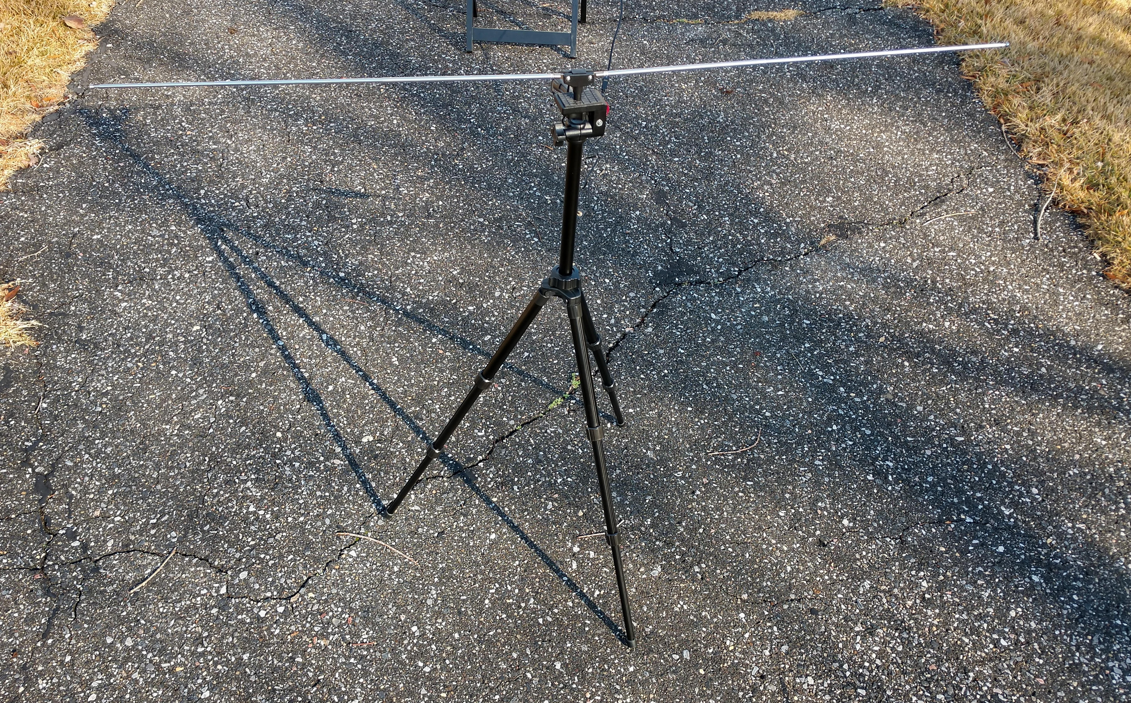
Yes, you need an antenna. Here's the thing.
- You don't need one of the dishes in NASA's Deep Space Network.
- You don't need this antenna.
- You don't need (as stated on the "Wxtoimg" website), "A good, special-purpose antenna... no matter what receiver you choose."
- You don't need to worry about the fact that the signal coming down from the satellite is circularly polarized.
- You don't need a QFH (quadrifilar helix antenna).
What do you need? Whichever antenna works for you. Quick digression. At this point, I tell people how a friend of mine told me the "perfect wine" story. To wit, what is the perfect wine for you? Whichever one you like. The analogy works for antennas. Whichever one works for your setup is maybe not your perfect antenna, but your good enough antenna. Yes, if you're going to be serious about collecting such signals, you can make a "quadrifilar helix antenna" (QFH). But if you just want to see some signals for yourself, then pretty much any antenna that works in the 137 MHz range should suffice. And how will you know it works? When you see and/or hear the signal from the GRC demodulated output. I'm using a basic "rabbit ears" set of whip antennas. Most likely, even a simple whip antenna would suffice. You might ask, "Would I get a better signal if I used a better antenna?" Yes. That's how RF works. "Better antenna" in this context would be "better gain towards the satellite" (kinda hard to do when the satellite is moving so quickly) and/or one that is circularly polarized. The bigger problem is not the antenna; it's the path loss due to trying to pick up the satellite when it's low on the horizon. In that case, the signal is having to work through and around houses and trees and cars and other objects. Being in the middle of an open field would be better. That gives you an unobstructed view towards the horizon. Another option? Put your antenna higher in the air. That has its issues, too. Mainly safety. Don't put an antenna high in the air when a thunderstorm is nearby. That. Would. Be. BAD!
The SDR
I used three different brand of RTL-SDRs while making this post. These were a Nooelec SDR Smart, a RTL-SDR Blog v3, and a Face2Face RTL-SDR. I obtained almost identical performance from the Nooelec and RTL-SDR Blog SDRs. The Face2face has an oscillator that is looser than the ones in the other two SDRs, but otherwise identical in performance.
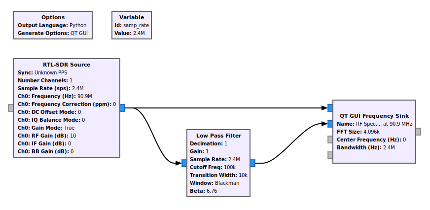
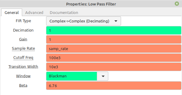
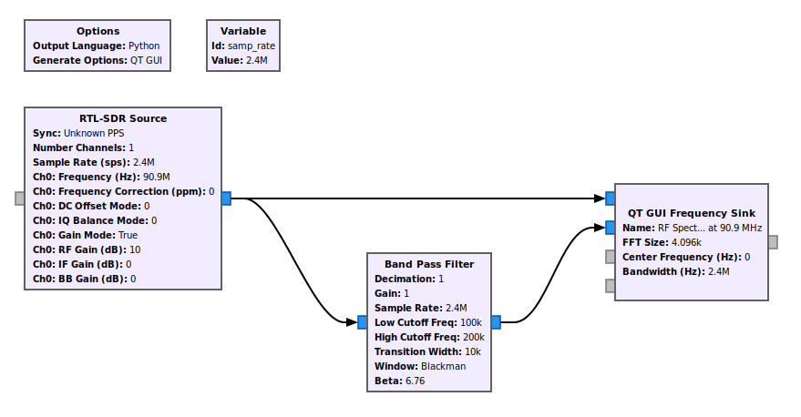
GRC Flowgraph
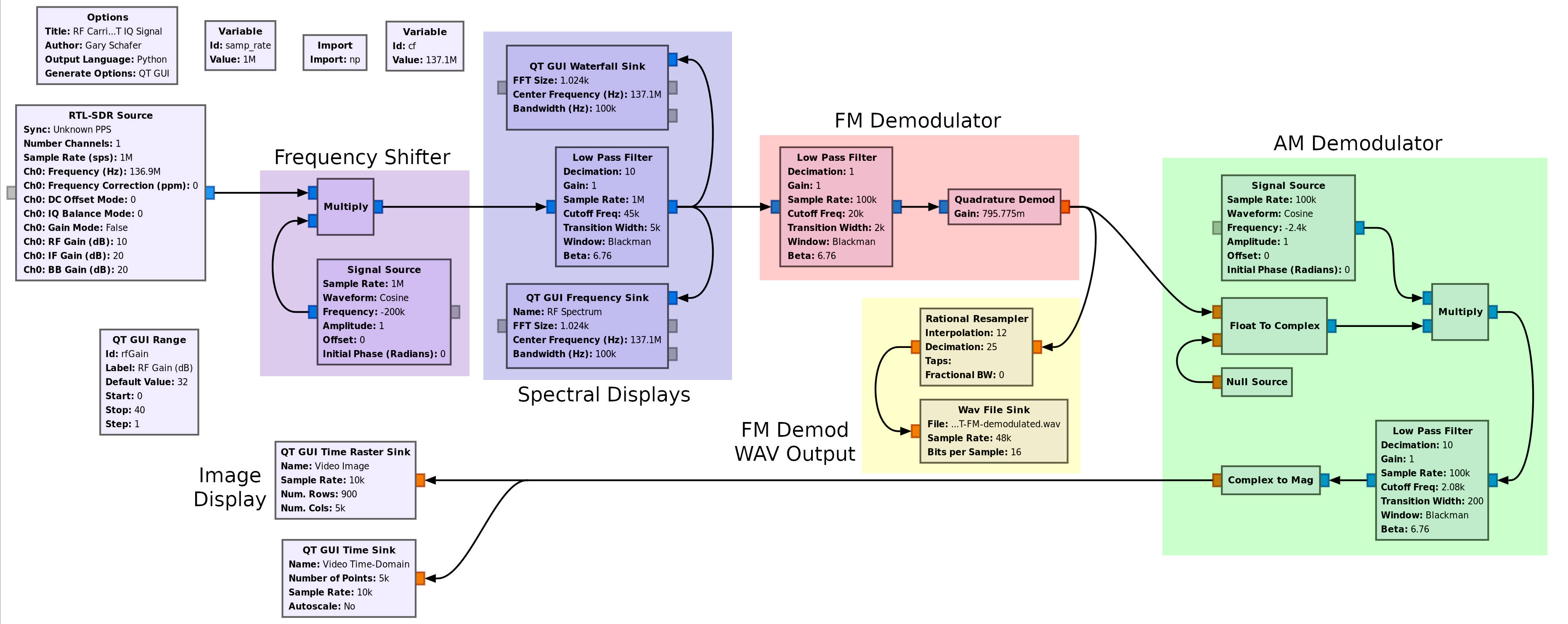
I go through the settings for the various blocks below. You can also download the GRC file itself (works on both GRC version 3.7 or 3.8), if you're so inclined.
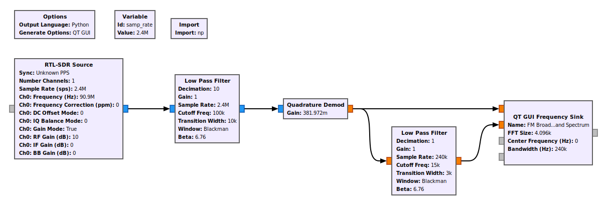
The SDR and Frequency Shifter
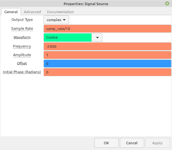
You can just take the output of the SDR and input it directly into the lowpass filter. The problem is "LO leakage". You know you have LO leakage when you look at the spectrum of your SDR output and you see a spike at the center. To help get around this, I add a "frequency shifter" at the output of the SDR. The SDR itself is set with a center frequency that is 200 kHz below the NOAA APT signal. This means that the NOAA APT signal will be 200 kHz above the center frequency. The "frequency shifter", consisting of a "Signal Source" block and "Multiply" block, shifts the spectrum down by 200 kHz. In other words, the SDR shifts the spectrum to the right, while the "frequency shifter" section shifts it to the left.
Yeah, if you're confused, don't feel bad. It takes a while to wrap your head around these ideas.


Spectral Displays
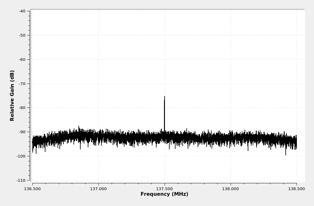
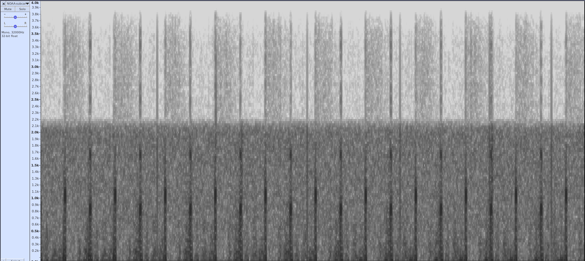
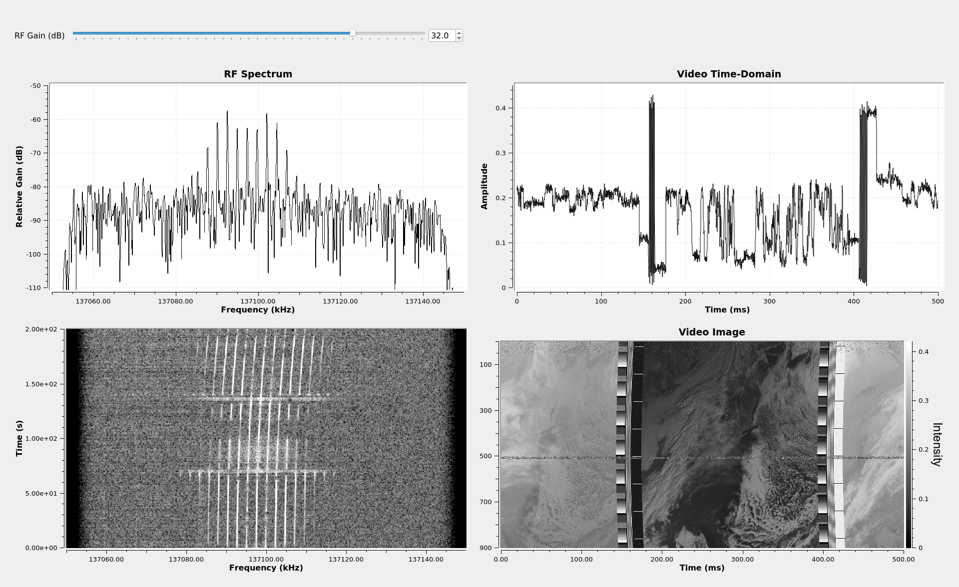
I'm used to having a spectral display for any signal I'm analyzing. The waterfall is actually better for determining when the signal is coming into view. The 2D display gives me an idea of how strong the signal is. I also prefer to see a bit of the spectrum around the signal I'm analyzing to determine if there are other signals that might be interfering. For that reason, I'm using a 100 kHz bandwidth for my spectral views.
Below is the spectrum of a NOAA APT signal I captured using the GRC "QT GUI Frequency Sink". This spectrum has a 100 kHz span and roughly 200 Hz resolution bandwidth (RBW).
Frequency Demodulator
The RF carrier is frequency modulated (FM) with a 17 kHz deviation. If you know anything about me and this website, it's that I've covered just about any frequency demodulator you can make with GRC. I could even argue that I've covered pretty much any frequency demodulator you can make digitally. These were covered in Post #1, Post #2 and Post #3.
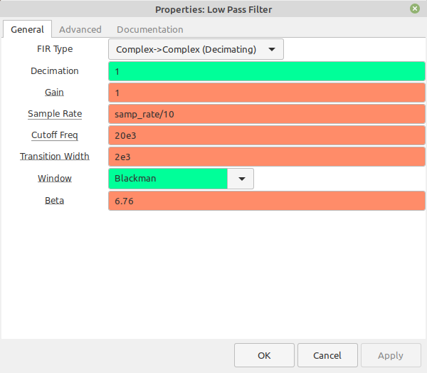
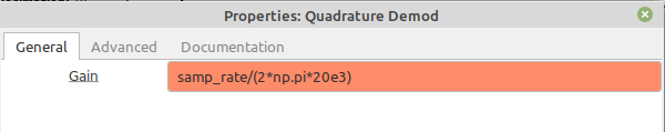
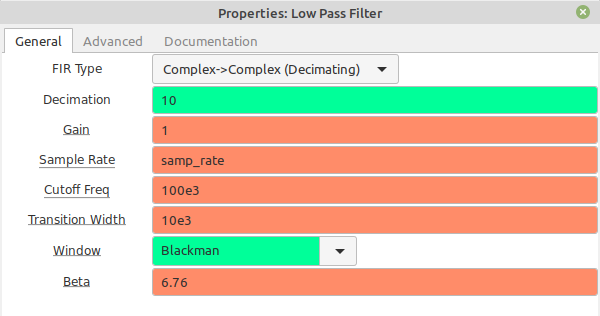
For this graph, we're just going to use the straightforward polar discriminator with the "Quadrature Demod" block. As always, we start by filtering the signal so that we're only demodulating the signal, and getting rid of as much noise and interference as possible. Remember: the signal is centered at 0 Hz. That's because we're using complex samples. A lowpass filter, in this case, will be a bandpass filter on our signal. We set the filter to include the deviation (17 kHz) plus some wiggle room for the Doppler shift, which can be upwards of 3+ kHz. This gives a deviation of +/-20 kHz.
If you want to use Martin Bernardi's "NOAA APT Decoder" program, you would create a WAV file of the frequency demodulated signal, then import that WAV file into the decoder program.
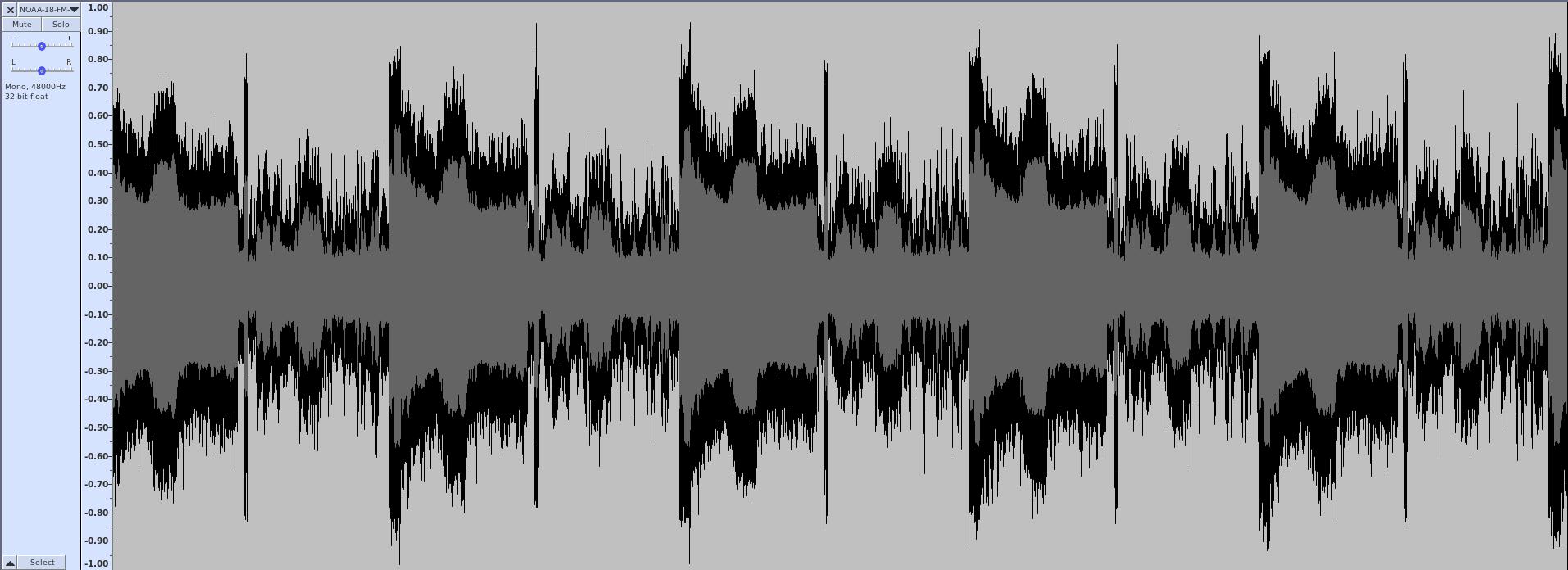
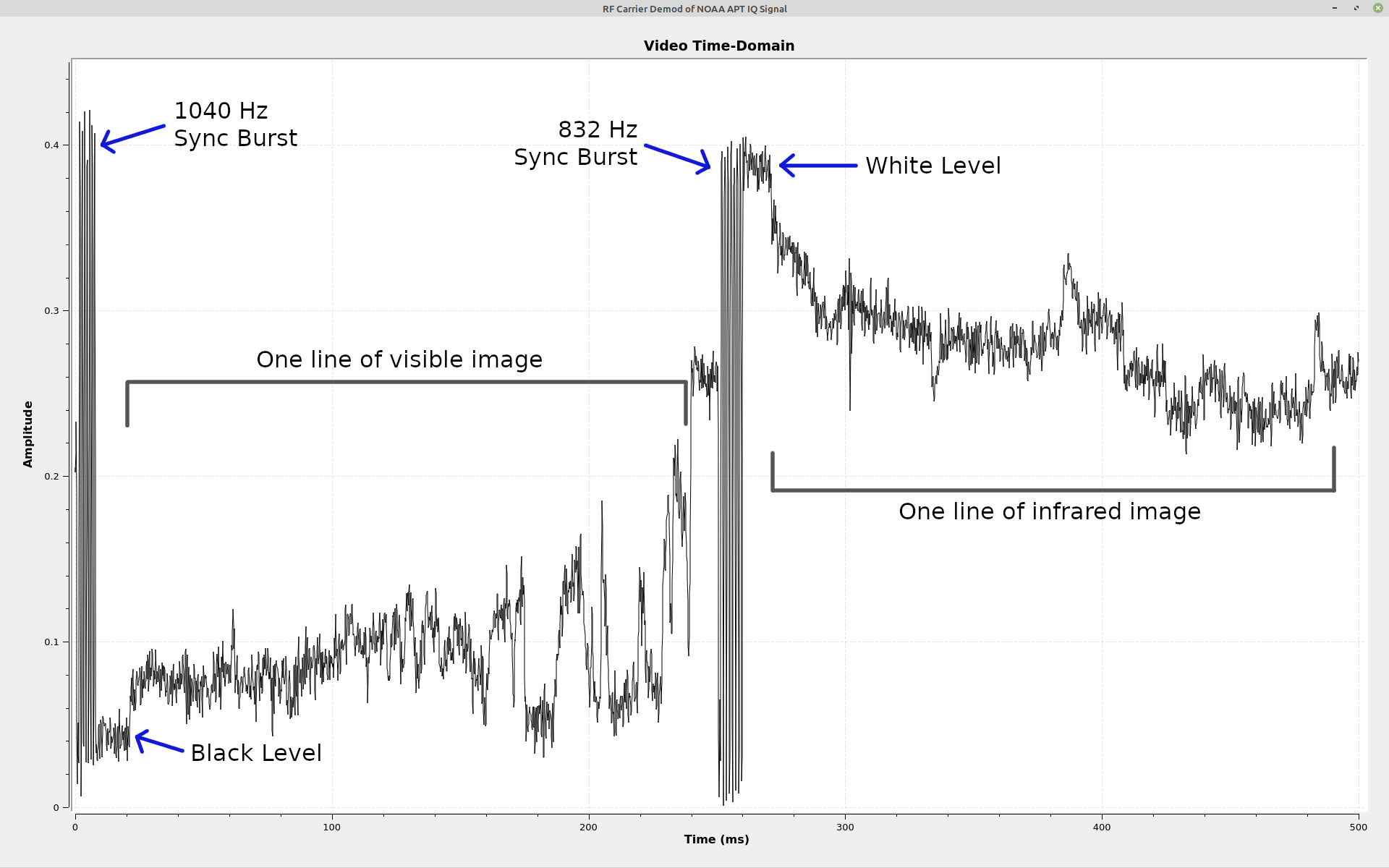
At this point, if you were to listen to the output when the signal is strong, you'd hear the following sound:
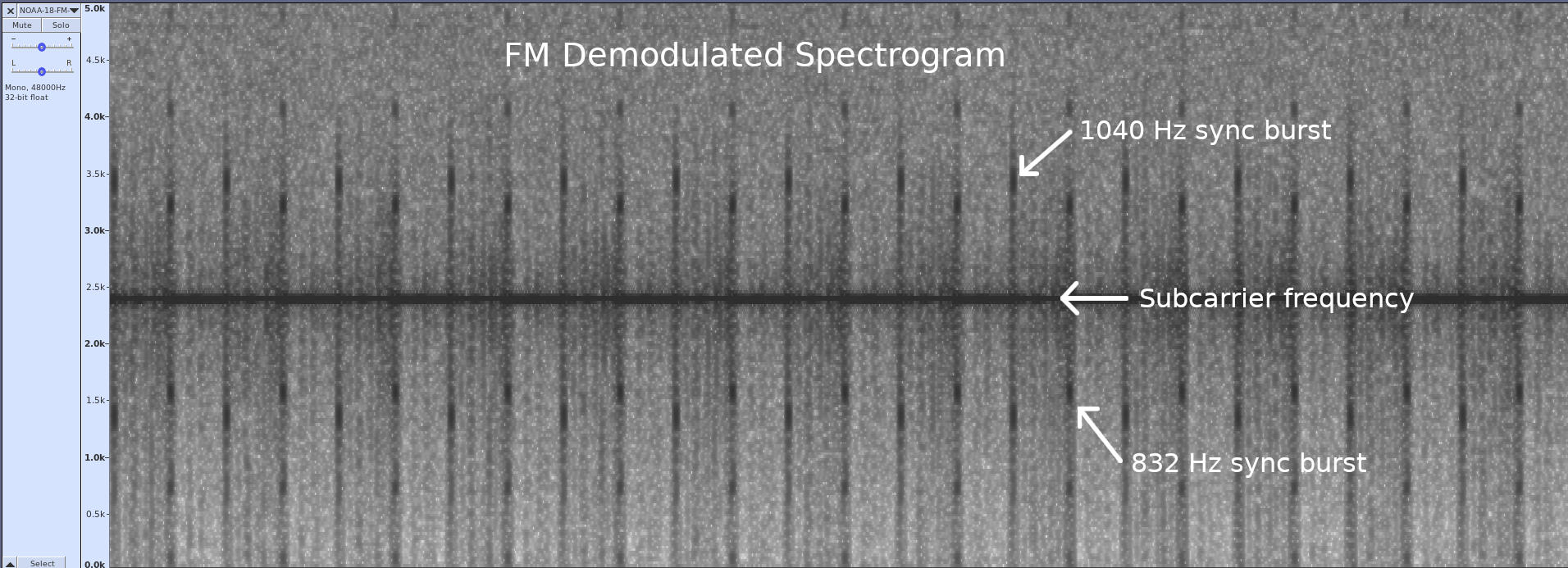
| FM demodulated audio from NOAA APT signal. The high-pitched whine is the 2400 Hz subcarrier. The "tick-tock" is the repetition of the 1040 Hz and 832 Hz sync bursts that each occur once every second. |
AM Subcarrier Demodulator
The APT signal is the video signal modulated onto a 2400 Hz subcarrier using double-sideband (DSB), full carrier (FC) amplitude modulation. To demodulate this signal, I'm using a modified "Asynchronous Complex Square-Law Envelope" detector. Unlike Dr. Lyons' suggestion, I'm not using a lowpass filter on the output. I've found that there's no discernible difference with and without the filter.
The first part of the "AM Demodulator" section converts the 2400 Hz real signal into a complex signal, then shifts it down to 0 Hz. The lowpass filter, again because it's operating on complex samples, bandpass filters the signal to a width of 4160 Hz (+/-2080 Hz). The "Complex to Mag" calculates the magnitude of each sample, which effectively amplitude demodulates the signal.

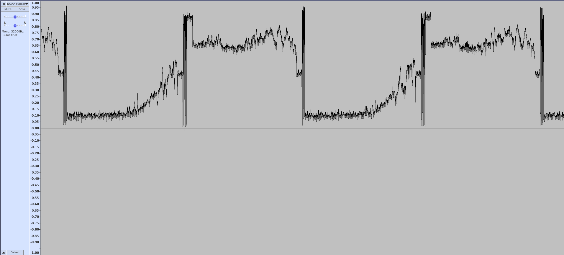
| Audio from the demodulated subcarrier. You still hear the "tick-tock" sounds of the 1040 and 832 Hz sync bursts, but without the high-pitched tone from the subcarrier itself. It also sounds muffled compared to the audio output direct from the frequency demodulator due to the fact that it has been filtered to just over 2 kHz. |
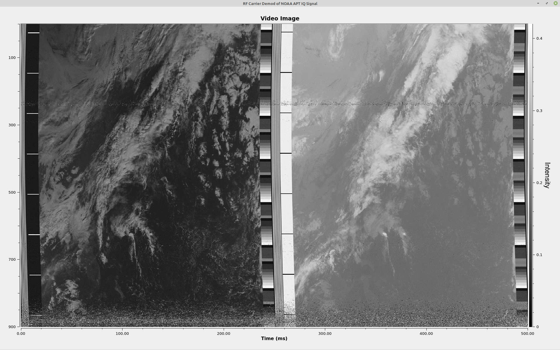
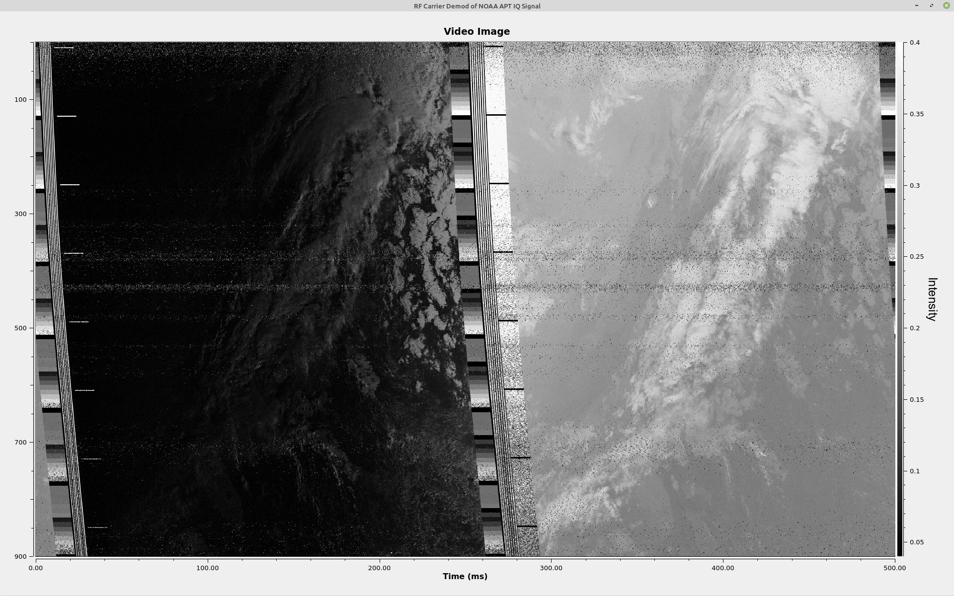
The Image Display
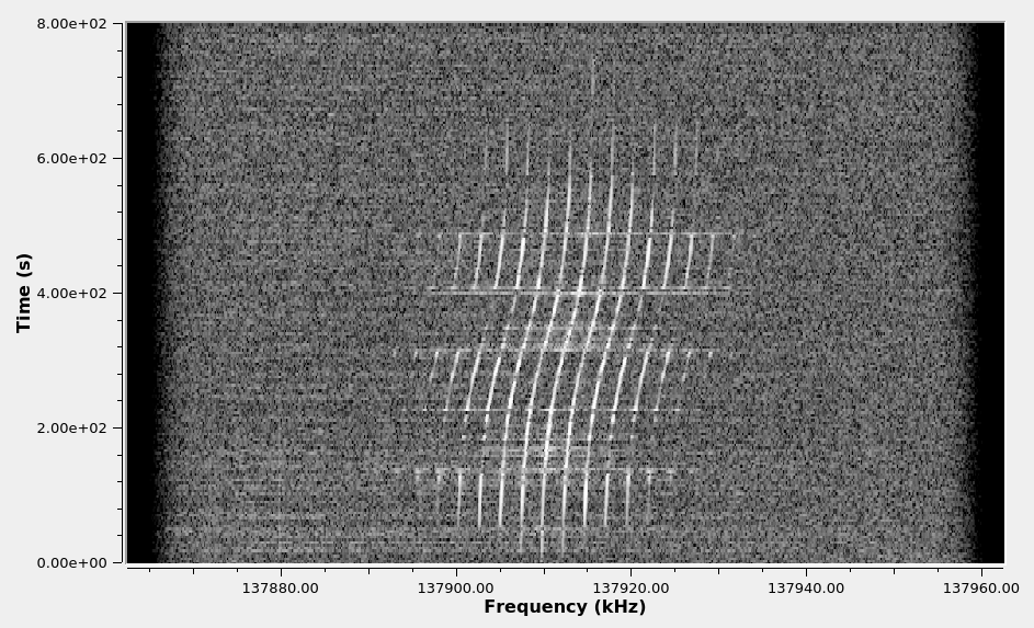
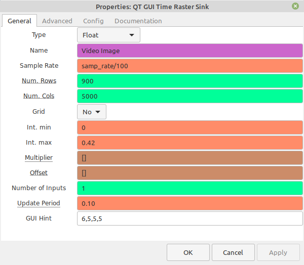
The whole point of the NOAA APT signal is to get an image. The various programs that you can use to get a pretty image will demodulate the subcarrier, synchronize each line of video, adjust the amplitudes so that the image goes from white to black using as large of a span as possible (to improve the image quality), and raster the image. We're just going to raster the signal. We're not going to use the signal itself for sync; we're just going to use the timing of the samples, which is based on the timing accuracy of the digitizer of your SDR. According to the NOAA information on the APT signal, each line is 0.5 seconds long. The output of the subcarrier demodulator is 10 kHz. If we set the number of columns to 5000, we'll roughly have the timing for an image. No, it will not be perfectly synchronized. As a matter of fact, if your SDR does not have a good oscillator, you may see a fair amount of drift from one line to the next. But you'll get a decent image.
As for the appropriate contrast, I eyeballed the white and black levels in the time-domain display, then set those as the maximum and minimum levels, respectively, in the time raster sink. That gave me a pretty decent image that even running through Gimp could not improve.
The Whole Thing
Here's the screen with all of the displays shown.
Next Steps
My next post will cover a bit more about GRC's filtering, this time covering the filters that require some Python code. After that, I'll probably go into all of the different forms of demodulation (AM, FM, PM).
Understanding Gnu Radio Blocks: Filtering
UPDATE: With special thanks to reader Chris G. for pointing out a math error, this page is (hopefully) correct now.
Now that I've beaten to death the different ways you can create a frequency demodulator in GRC, I thought I'd step back and take a look at some basic signal processing functions and how you perform them in Gnu Radio Companion (GRC). Let's start with filtering. If you don't understand filtering, signal processing becomes well-nigh impossible.
A lot of the knowledge for this post didn't come from either my undergraduate or graduate classes. It came from two books. These are Richard Lyons's "Understanding Digital Signal Processing" and Steven Smith's "Digital Signal Processing". Smith's book is even available for free as a PDF download (on a per-chapter basis, not the whole book at once). These books are expensive, but if you're looking for texts that actually explain the underlying concepts of digital signal processing, these are your starting point.
Filtering Overview
Filtering is the most-oft used form of signal processing. GRC not only provides explicit filter blocks, it is also built into many other GRC blocks. For example, several of the frequency demodulator blocks (FM Demod, NBFM Receive, WBFM Receive) also include not only frequency demodulation, but filtering as well.
The filters we're going to discuss are frequency-selective filters. There are four basic filter blocks we'll cover. The specific blocks we're going to cover are:
- "Low Pass Filter": Allows low frequency signals to pass through, and removes high frequency signals.
- "High Pass Filter": Allows high frequency signals to pass through, and removes low frequency signals.
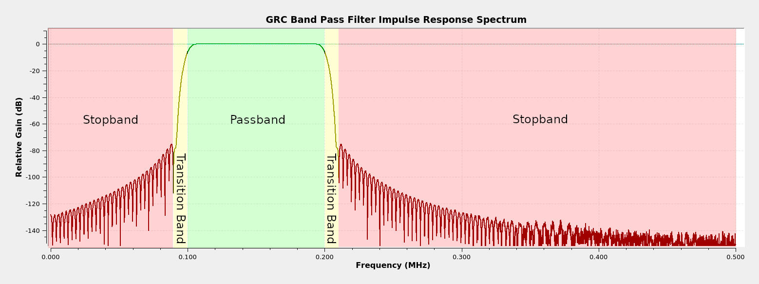
- "Band Pass Filter": Allows signal within a defined band to pass through, and removes signals that are outside of the band.
- "Band Reject Filter": Removes signals within a defined band, and allows signal outside of the band to pass through.
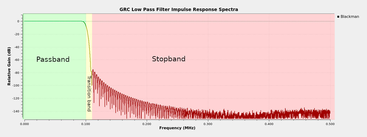
A filter is divided into three, basic sections. These are as follows:
- Passband: The passband is the section of the filter where the signal is either not attenuated, or attenuated only minimally.
- Stopband: The stopband is the section of the filter in which frequencies are attenuated to the greatest degree possible. Essentially, this is the section of the filter in which signals are removed.
- Transition band: This is the section between the passband and stopband. It's impossible to go directly from passband to stopband. The width of the transition band (which GRC calls the "transition width") determines the selectivity of the filter. From a practical sense, the ratio of the transition width to the sample rate determines the amount of processing required. The smaller this ratio, the more processing required. This is because, the smaller the ratio, the sharper the filter. In the analog days, a sharp filter required more components or a more complicated structure; in the digital realm, it requires more processing.
FIR vs IIR
If you study digital signal processing and filtering, you find out that filters come in two forms. These are finite impulse response (FIR) and infinite impulse response (IIR). The difference between them is that IIR filters use feedback, while FIR filters do not. This means that IIR filters have to be carefully designed; otherwise, they could be unstable. This means that the algorithms for designing IIR filters are more complicated than those for FIR. The advantage of IIR filters is that they tend to be easier to process (fewer computations required).
All of the filters on this post ("Low Pass", "High Pass", "Band Pass", "Band Reject") are FIR. This is why you'll see the term "FIR Type" at the top of the "Properties" window for each of these filter blocks.
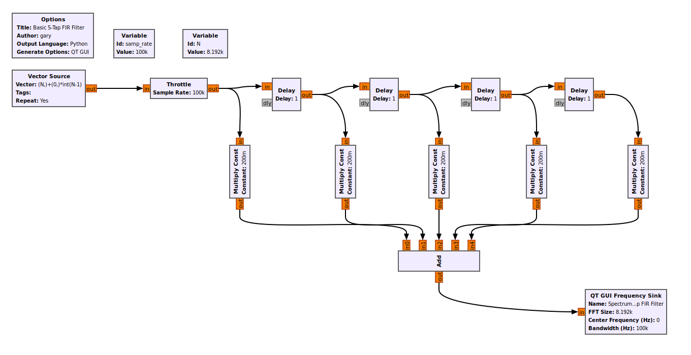
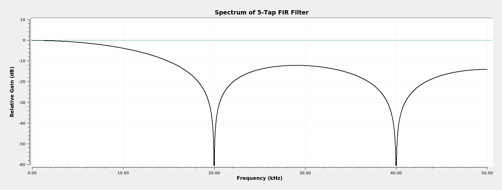
We can use GRC to create a basic FIR filter. A FIR filter is, essentially, a combination of delays and multiply blocks. This is a simple, 5-tap filter that averages the input. Each "Multiply Const" is a "tap", and the "Constant" value in each block is the "tap coefficient". The GRC filter blocks that we'll cover will create filters that may have hundreds of taps. This is a simple example so that you understand a FIR filter and the terms "tap" and "tap coefficient".
Float (Real) vs Complex
If you want to truly understand digital signal processing, you really have to understand complex signals. I'm not going to provide any kind of deep background on complex signals. I will provide the following bullet points, though:
- Complex signals have both positive and negative frequencies. Actually, so do real signals (which GRC calls "floats"). But in real signals, the positive and negative frequencies are identical.
- The positive and negative frequencies are different in complex signals. In real signals (again, which GRC just calls "floats"), the two sides are identical (though their respective negative and positive frequency components are complex conjugates of each other).
- In GRC, a blue connector is complex samples. An orange connector is real ("float") samples.
There is one thing you need to understand about filtering. There are complex samples and there are complex tap coefficients. The samples are what gets filtered; the tap coefficients determine whether the filter will operate on both sides equally (real taps) or can operate on each side uniquely (complex taps). I'll point out where this makes a difference as we go.
NOTE: If the filter does not explicitly state whether the taps are real or complex, then the taps are real.
How GRC Creates Filters & The Windowed-Sinc Method
Again, we're talking about four filter blocks. These are "Low Pass", "High Pass", "Band Pass", and "Band Reject". These four filters are all FIR filters. GRC calculates the tap coefficients for these blocks using the windowed-sinc method. Starting with the "Low Pass" filter, there are four steps:
- Calculate the number of taps required for the filter using the "harris approximation".
- Calculate the base sinc pulse using the number of calculated taps.
- Calculate the window values.
- Multiply the sinc pulse with the window on a point-by-point basis. The values of the windowed sinc pulse are the tap coefficient values.
A lowpass filter is the basis for all of the other filters. We can create a highpass filter from the lowpass filter values above by subtracting it from an impulse. We can create a bandpass filter by creating an appropriate lowpass and highpass filter, then calculating the convolution of the impulse responses of the two filters. This sounds complicated. When I say "impulse responses", since we're talking about FIR filters, the impulse response amplitudes are the same as the "tap coefficients" for our filter.
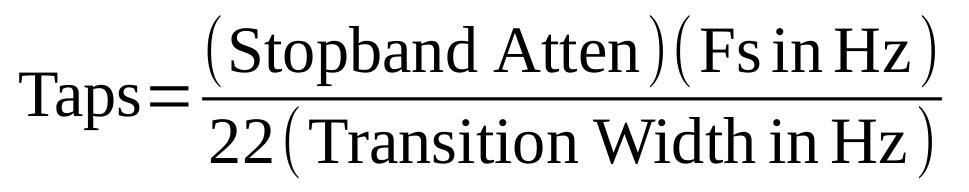
Calculate the Number of Taps
GRC calculates the number of taps using the "harris approximation". The equation is below.
The table below compares the different windows and their stopband attenuation values.
| Windowed-Sinc Filter Minimum Attenuation in Stopband | |
|---|---|
| Filter Window | Stopband Attenuation, Minimum (dB) |
| Rectangular | 21 |
| Hann | 44 |
| Hamming | 53 |
| Blackman | 74 |
| Kaiser (Beta = 6.28) | 65 |
| Kaiser (Beta = 6.76) | 70 |
| Kaiser (Beta = 9.42) | 94.0 |
| Kaiser (Beta = 15.71) | >140 |
As an example, with a sample rate of 2.4 MHz, a transition width of 10 kHz, and a Blackman filter (stopband attenuation of 74), we calculate the number of taps as (74)(2.4 x 10⁶)/(22*10 x 103) = 808 taps (rounding up).
Create the Sinc Pulse
For the rest of this example, I'm going to use Gnu Octave to calculate the various values as well as plot the graphs. If you have Gnu Octave loaded, you can download the file yourself and run it, if you're so inclined.
With the number of taps, the frequency cutoff, and the sample rate, we can calculate the sinc pulse. The "sinc", or "sine cardinal", is a quickly decaying sinusoid. The equation used to calculate the sinc pulse is:
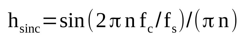
The equation for calculating the sinc pulse, where:
- N = number of taps
- n = counter used to calculate sinc pulse, with -N/2 ≤ n ≤ N/2.
- fc = the cutoff frequency
- fs = sample rate
Note that, when n = 0, you have a "divide by zero" problem. The value hsinc(0) should be set to 2fc/fs.
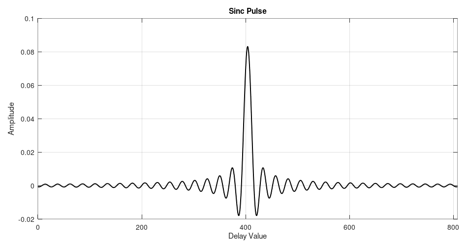
Sticking with our example of a lowpass filter with a sample rate of 2.4 MHz, a cutoff frequency of 100 kHz, and a 808 tap filter, we get the following sinc pulse:
Create the Window
The filters discussed here allow for five possible windows. These are "Hamming" (the default), "Hann", "Blackman", "Rectangular", and "Kaiser". Let's go through them briefly.
The "Rectangular" window is really no window at all. This type of window, also called a "uniform" or "boxcar" window, really means you're not using a window. For a windowed-sinc filter, this means you're using a sinc pulse, and that's it. It provides the least amount of attenuation in the stopband (21 dB), but as a result, it also requires the least amount of processing.
The "Hann", "Hamming", and "Blackman" windows are standard windows. You can see how they are generated by reading fred harris's original paper on digital windows. While the Gnu Radio documentation on windows states that many of the windows are based on information provided in the Oppenheim and Schafer (no relation) text "Discrete-Time Signal Processing", harris's paper also provides the background for these various windows.
The last window, "Kaiser", is a special form of window. It has a parameter, called a "beta" value, that allows its attenuation to be adjusted. With the other windows, the attenuation is fixed. With a beta value of 1, the Kaiser-based lowpass filter is roughly equivalent to the "Rectangular" window filter. Also of note is that, with the first, four windows, you can get stopband attenuations of 21 - 74 dB. With the Kaiser window, you can have attenuation values greater than 140 dB.
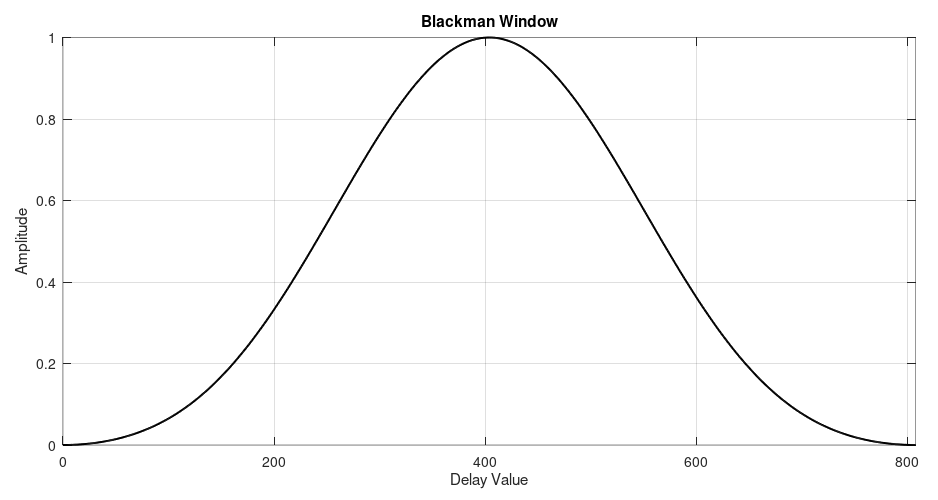
For our example, we're using the "Blackman" window. We need a Blackman window made of 809 taps. (NOTE: The original value was 808, but we added one more for the zero index.) The equation for the Blackman window is:
w(n) = 0.42 - 0.5*cos(2*π*n/N) + 0.08*cos(4*π*n/N)
where:
- w = window values
- N = number of taps
- n = counter for calculating the window values, 0 ≤ n ≤ N.
The graph for this particular window appears as follows:
Multiply Sinc Pulse with Window
By multiplying the sinc pulse with the window, we get the final windowed sinc pulse. The values used to create this graph are the "tap coefficient" values used for the FIR filter.
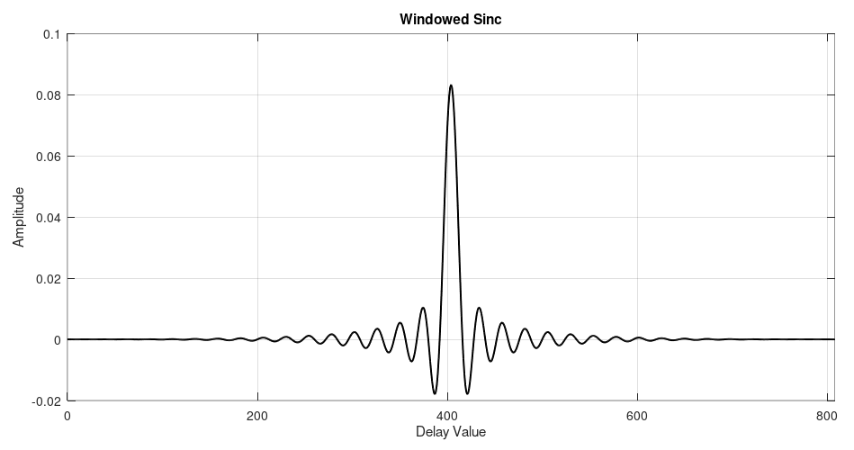
Here's the spectrum of this lowpass filter.
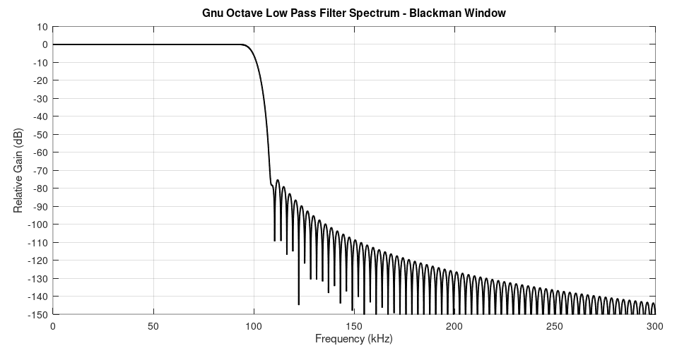
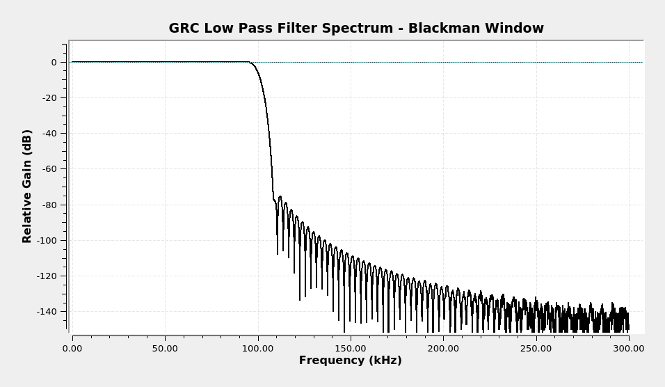
Here's the spectrum of the filter in GRC so that you can compare it with the filter calculated with Gnu Octave above.
Once GRC has calculated the tap coefficients, it uses one of two methods to actually filter the signal. It either uses a straight time-domain convolution or a frequency-based (FFT) convolution.
Filter Examples
Let's look at some examples of various windowed-sinc filters. I'm going to use some FM broadcast stations to demonstrate both the windowed-sinc filters as well as the different types of filters (lowpass, highpass, bandpass and bandreject).
We're going to start with a spectrum of part of the FM band. I captured this using a RTL-SDR centered at 90.9 MHz and a 2.4 MHz sample rate.
Complex Sample Lowpass Filter
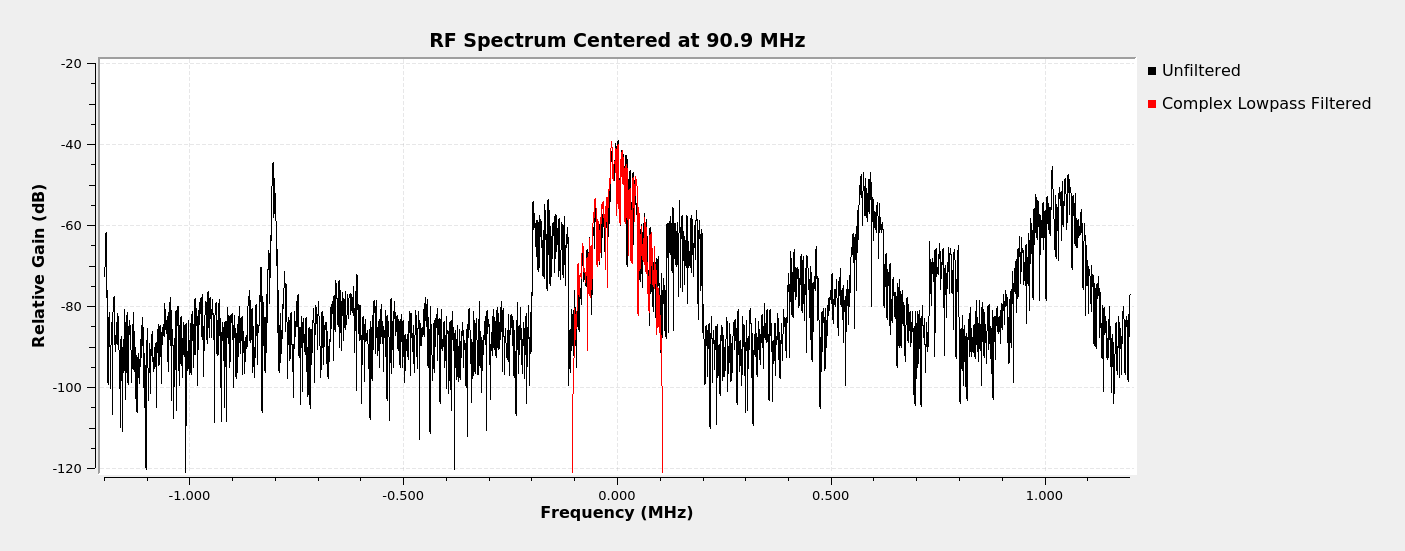
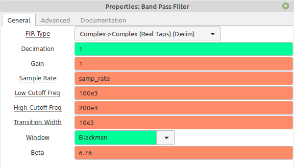
Complex Sample Real Tap Bandpass Filter


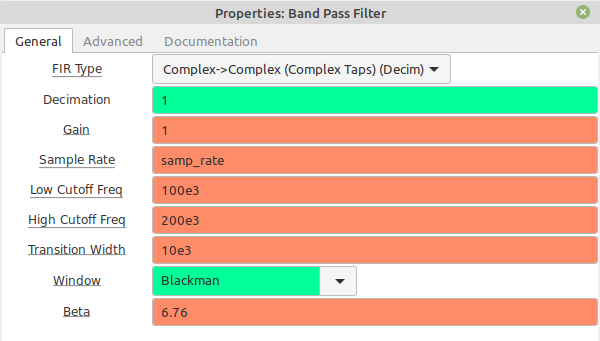
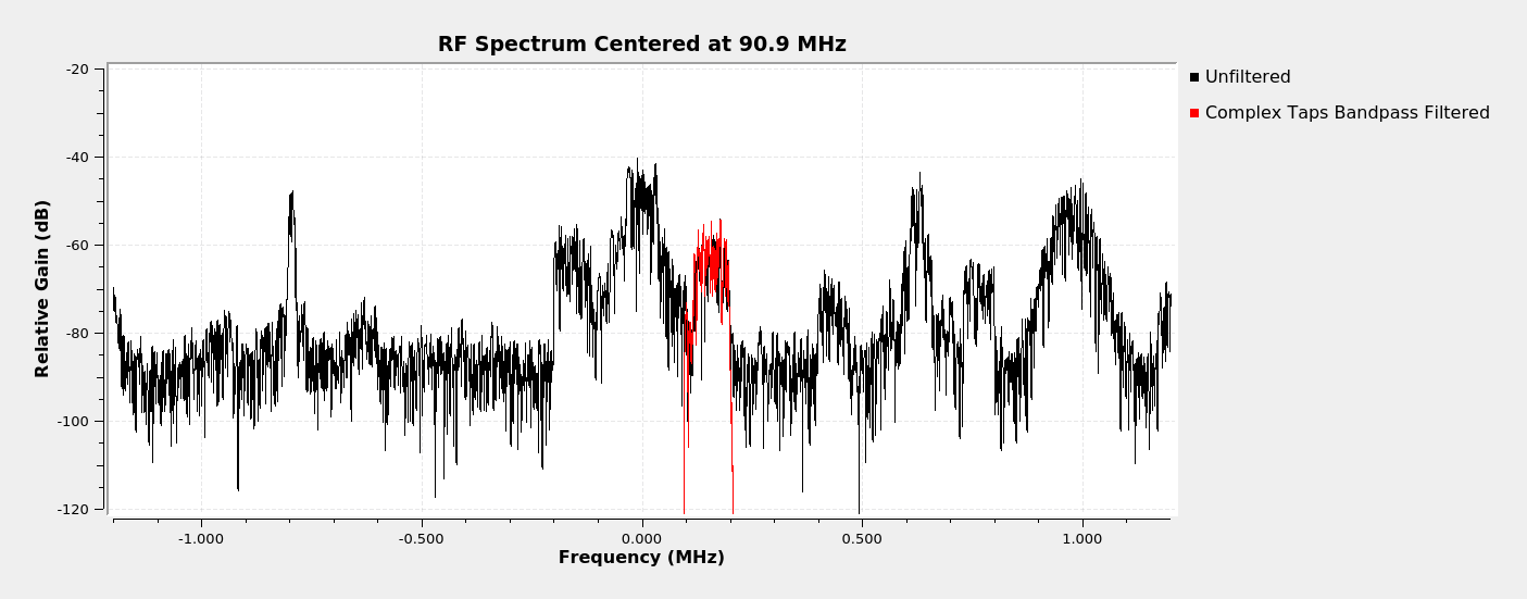
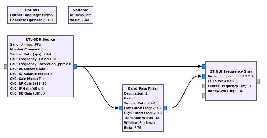
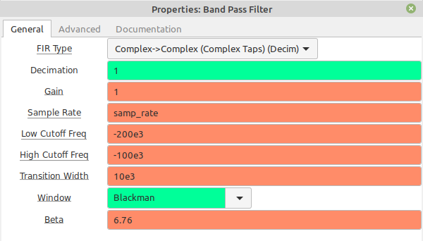
Complex Sample Complex Tap Bandpass Filter
Okay, here's where we can go a little nuts with our frequency limits. The "Band Pass Filter" block allows you to select either real taps or complex taps. Again, real taps means the signal will operate equally on both positive and negative frequencies for complex samples. But complex taps can operate differently on positive and negative frequencies.

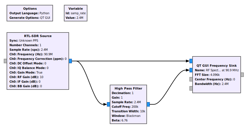
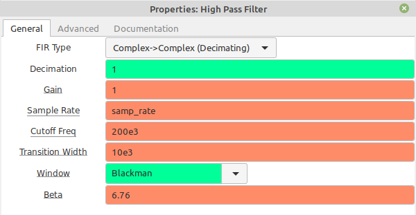
Complex Sample Highpass Filter
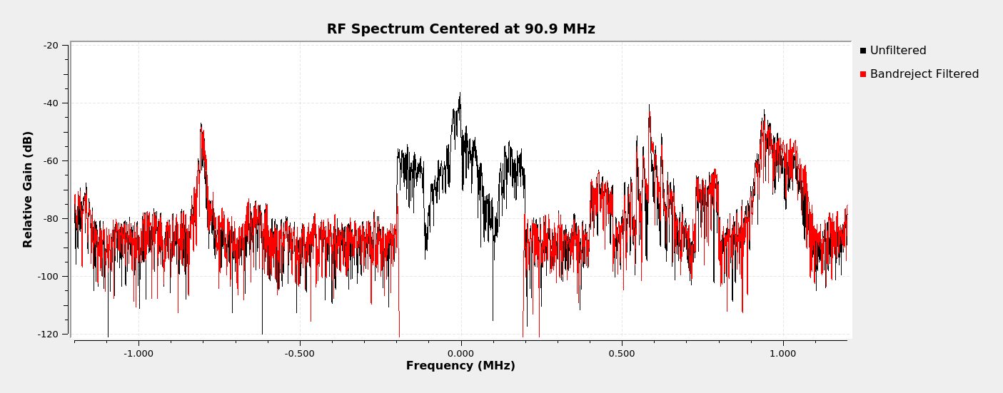
Just as a complex sample lowpass filter can effectively be a bandpass filter, a complex sample highpass filter can effectively be a band reject filter.
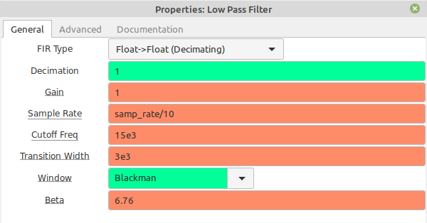
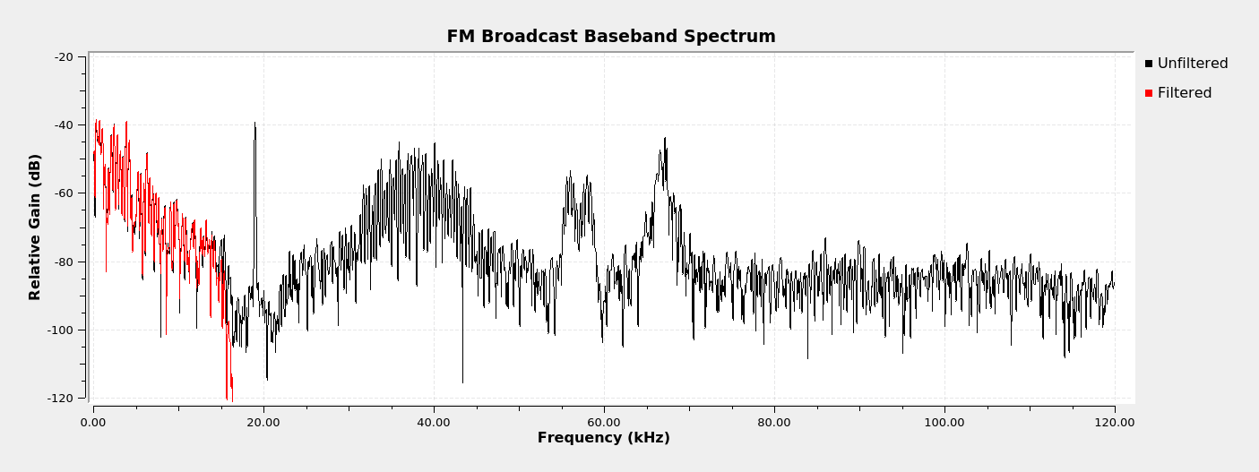
Real Sample Lowpass Filter
We're going to start with the complex sample lowpass filter which extraxts the analog FM broadcast signal. We can pass that through a frequency demodulator to get the baseband spectrum.

Next Steps
I'd originally started this post to talk about filtering, demodulation and decimation / interpolation. That turned into a veeeeeeeeery long post. So I shortened it just to filtering. Then that turned into a veeeeeeeeeeeeery long post, so I shortened it just to these four filters.
What that means is that I'm now working on covering filters using the various Python command line functions. I'm also working on a post on demodulating NOAA APT signals as well as how to create a stereo receiver. The point of these posts is to allow you to create these receivers using the basic components already available in GRC. I want you to understand what's going on, not just "connect blocks together".
That will be for next time.