Gnu Radio & Frequency Demodulation - One More Time

Gary Schafer, Blursday, Pandemic Time, Maybe May 2020

If you're here to find a basic FM receiver because you're just getting started with SDRs and Gnu Radio Companion, I have you covered.

As a I said in my last post, I went deep down the rabbit hole in trying to understand how Gnu Radio Companion's frequency demodulator works.

I wound up trying to answer the question, "How many different ways can you make a frequency demodulator in Gnu Radio Companion?" Turns out, quite a few. I'm just going to document them here. I'm going to go through these different methods roughly historically.

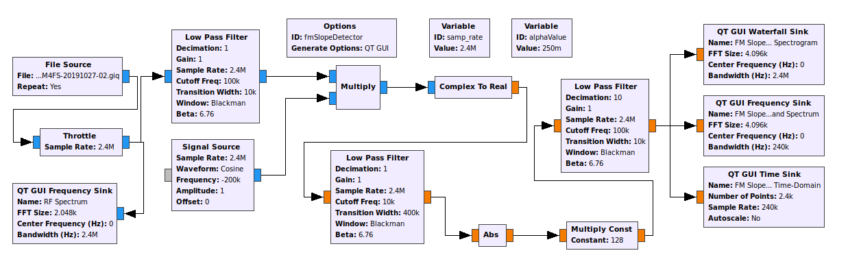
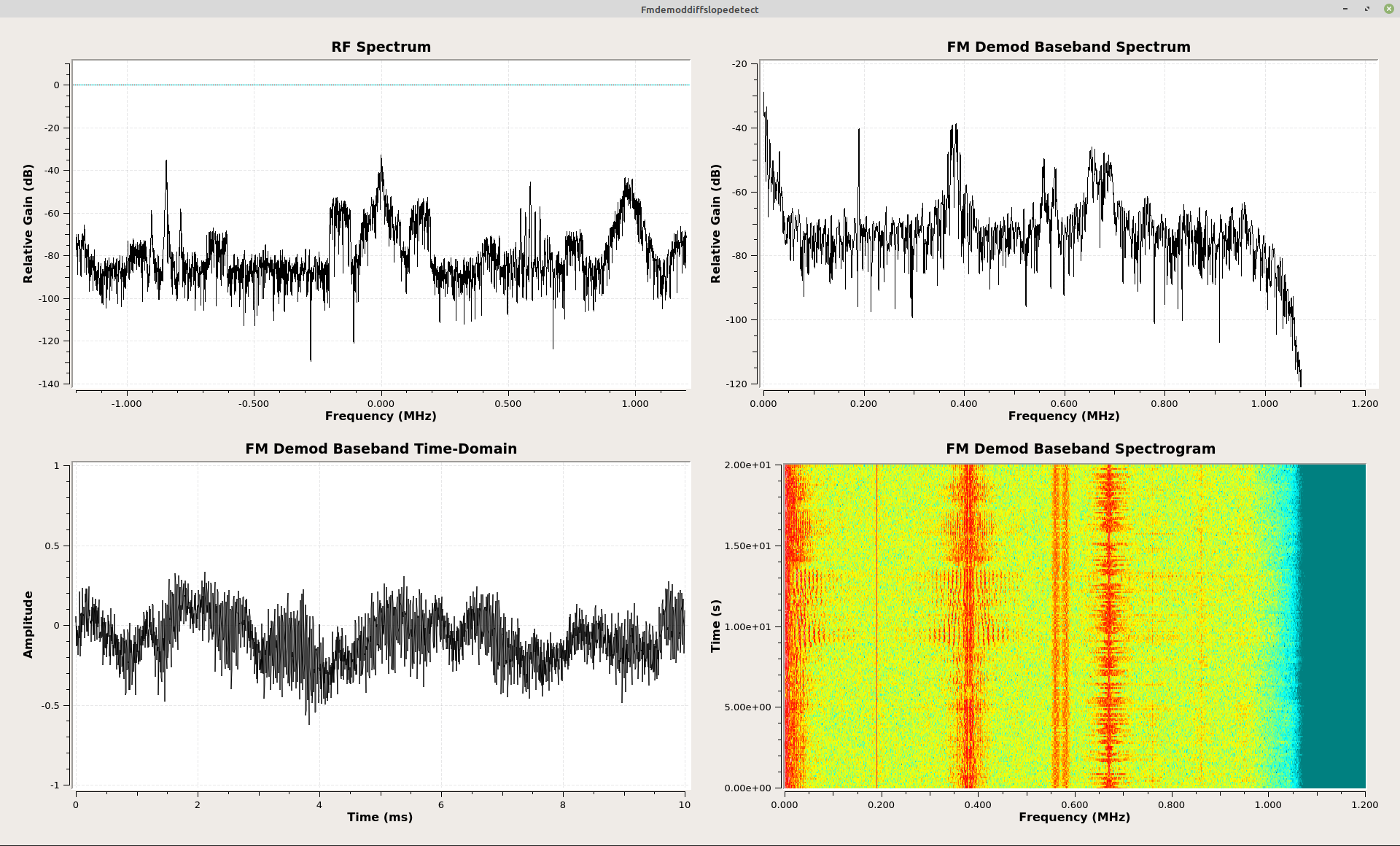
The Slope Detector

I'm going to start with the old, analog days. One of the first frequency demodulators used^{[CITATION NEEDED]} was a "slope detector". The idea is this. A frequency modulated (FM) signal will vary its center frequency in concert with the amplitude of the modulating signal. As the modulating signal goes higher in amplitude, the FM signal will increase in frequency. And vice-versa. If you have a filter whose amplitude vs frequency is a slope over the frequency range of the FM signal, then the output of the filter will be the FM signal, but also amplitude modulated with the same information. Now it can be demodulated the same as any AM signal.

GRC graph for a slope detector. The input is a stream of complex samples. It is shifted to -200 kHz, then converted to real samples. This has the effect of inverting the spectrum. This real signal is passed through a lowpass filter, which varies the amplitude of the signal in concert with the information. This "slope detects" the signal. The filtered signal is passed through a "Abs" block. This envelope detects, or amplitude demodulates, the signal. The final lowpass filter removes all of the extraneous signals due to the "Abs" block. The output is the final frequency demodulated signal.

Time-domain and frequency-domain graphs for the input and output of the slope detector.

The Differentiator and Envelope Detector

Mathematically, the slope detector is equivalent to a differentiator followed by an envelope (AM) detector, as shown below.

Block diagram for FM discriminator using a differentiator followed by a envelope detector. (From "Principles of Communications: Systems, Modulation, and Noise (Second Edition)", R.E. Ziemer, W.H. Tranter, Houghton Mifflin Company, 1985)

What do computers do really well? Math. GRC provides all of the components necessary to make such a demodulator directly. This is shown below, along with the resulting time- and frequency-domain graphs.

GRC graph for differentiator-and-envelope-detector FM discriminator. The input is a stream of complex samples. To convert these to real, they have to be frequency shifted so that no part of the signal bandwidth passes through 0 Hz. Since the signal is 200 kHz bandwidth (+/- 100 kHz), the signal is shifted to a center frequency of 200 kHz. The signal is then converted to real by the straightforward measure of throwing away the imaginary component and keeping the real part (using the "Complex to Real" block). The differentiator is a delay and subtract block set. By subtracting the delayed, sample from the current sample, this is a first-order differentiator. This is followed by an envelope detector, which is a combination of the "Abs" (absolute) block and lowpass filter. The two blocks in between simply serve to remove the DC component and to amplify the signal.

Time- and frequency-domain graphs for the differentiate-and-envelope-detect discriminator.

The Foster-Seely and Ratio Discriminators

I looked at mimicking both a Foster-Seely and ratio discriminators using GRC. They're both based on using transformers. Both of these circuits operate by varying the lead and lag of the current with the voltage. I've not been able to figure out how to mimick this with GRC. On to the next one.

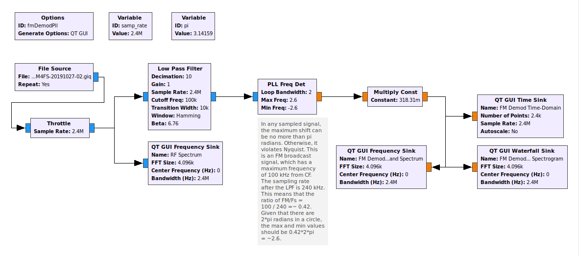
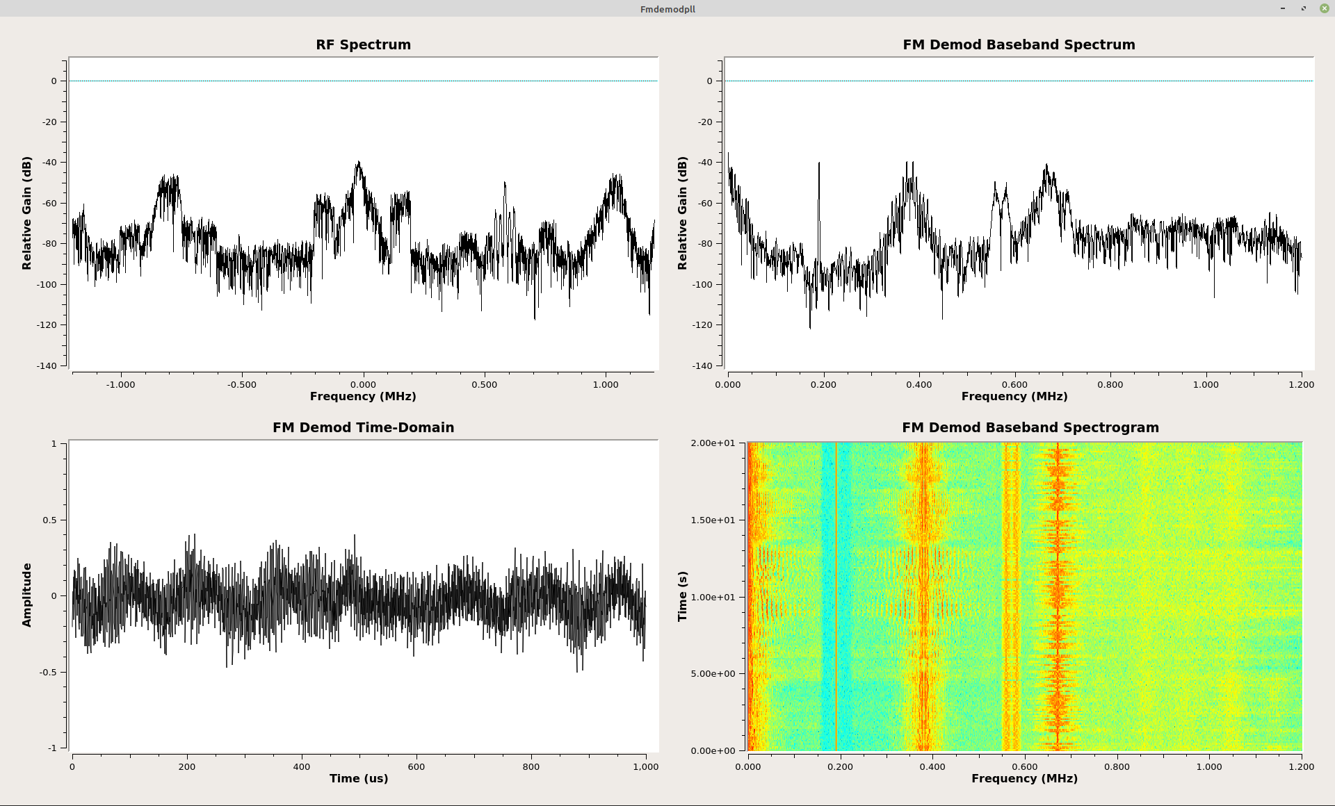
The Phase Lock Loop (PLL) Demodulator

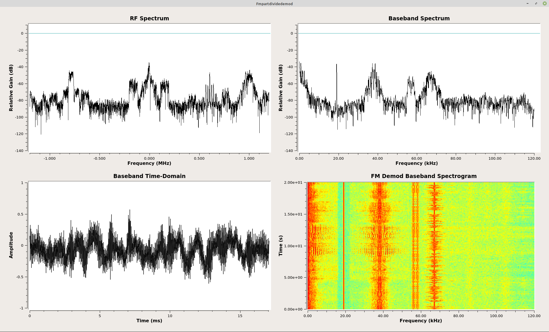
The phase lock loop (PLL) is the only circuit that requires a feedback loop. GRC does not allow loops between blocks. However, GRC does provide a PLL block, in this case the "PLL Freq Det" block. Here's the problem. The "PLL Freq Det" block does not use normal units for the minimum and maximum frequency. Rather, they use units of "radians/sample". What does that mean? We're talking about sampled signals. FM signals will have phases that are changing with each sample. The phase difference per sample will depend on the quotient of the frequency deviation divided by the sample rate. Phase can be measured in one of three units. These are radians, gradians, and degrees. Radians allows for easier math. So that's what is used more often. The phase change per sample, in radians, is nothing more than this quotient multiplied by 2π. For this example, the sample rate at the input of the PLL block is 2.4 MHz (the sample rate) divided by 10 (the lowpass filter decimation value) = 240 kHz. The deviation of an FM broadcast signal is 75 kHz. However, to ensure that there's no overload, I increased this to 100 kHz. The ratio is thus 100 / 240 = 0.4167. The value in radians/sample is 0.4167*2π = ~2.6 radians/sample. This corresponds to both plus and minus. These are the values that are in the "PLL Freq Det" block.

GRC graph using a phase lock loop (PLL). Since GRC does not allow feedback between blocks, the only way to incorporate it is to program into the block itself. All of the feedback occurs within the block itself. The values for the block ("Loop Bandwidth", "Min Freq", "Max Freq") are based on units of "radians/sample", rather than "Hz". Also, since the samples are complex, the "Min Freq" can be negative. Given this is a FM broadcast signal (+/- 100 kHz), to convert this to radians/sample, divide by the sample rate, then multiply by 2π. This gives a value of 2.6 radians/sample. The same thing goes for the "Max Freq" value. As for the "Loop Bandwidth", I'm still trying to figure out what value is ideal for that one. The value here ("2") works, and that's enough for now.

Time-domain and spectral graphs for FM discriminator using a phase lock loop (PLL).

Zero-Crossing Discriminator

Yet another of the techniques that I've not yet figured out how to mimick in GRC. Nuf said.

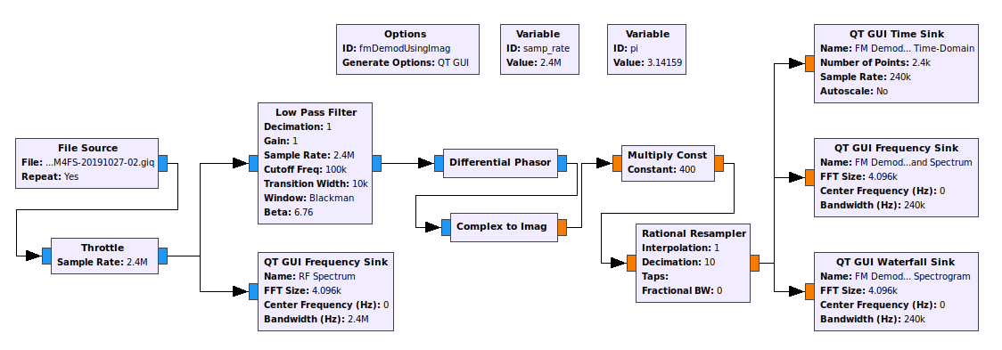
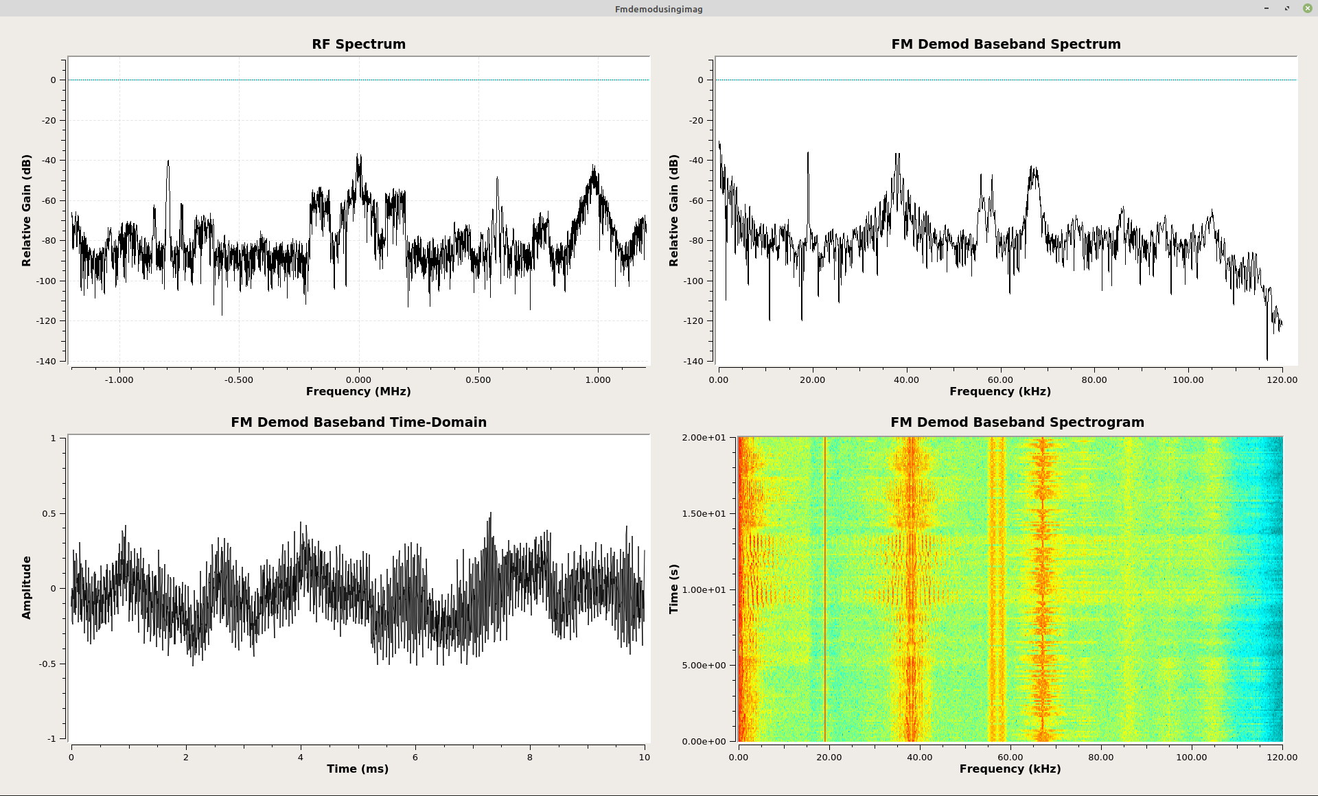
Phase Differential

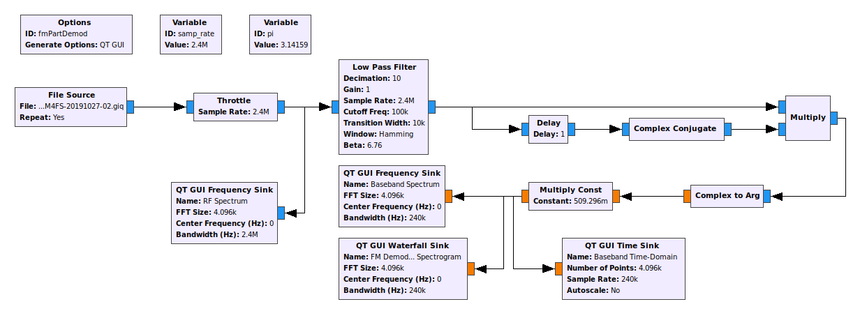
This goes back to the original idea of a frequency demodulator. Frequency is nothing more than the change of phase over time. The basic idea, then, is to measure the phase of the FM signal at each point, then subtract the phase between consecutive samples. Putting this together straight in GRC gives the following:

This graph takes each sample and calculates the phase of each (using the "Complex to Arg" block). The following "Delay" and "Subtract" blocks calculate the phase difference between samples. The problem is that, the "arg" function only provides values that are between +/-π. If the consecutive samples straddle this line (for example, one that is near +π and the other near -π.), then the difference will be near +/-2π. This creates a bunch of impulses (seen in the time-domain view of the output).

This is the time-domain and spectral graphs of the output of the phase difference graph. The time-domain graph shows impulses when the consecutive samples fall across the +/-π line. These impulses make the output useless. There are two ways to get rid of these once they're created. The first is to put an "if/then" decision after each subtraction. If the absolute value of the phase difference is greater than π, adjust it so that it falls between +/-π. The second option is to convert the phase back to Cartesian coordinate complex samples, then re-calculate the phase.

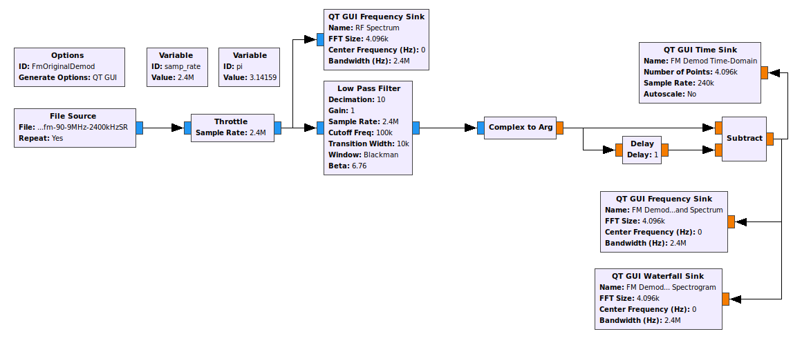
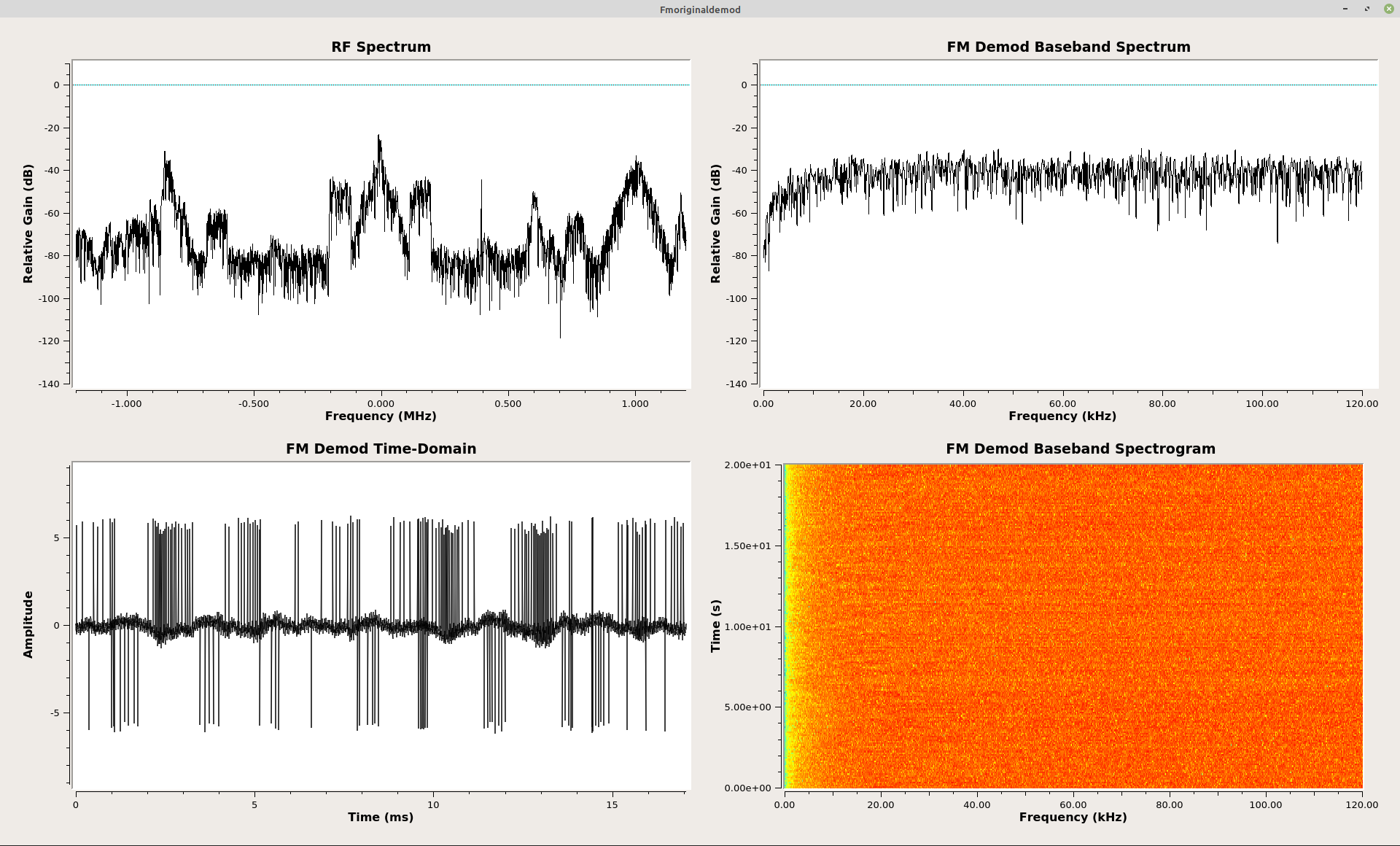
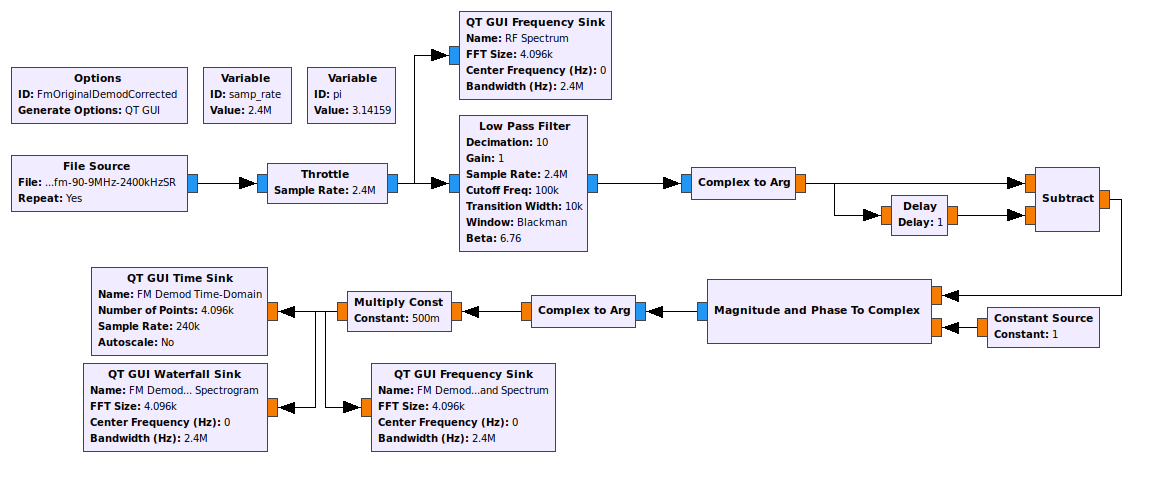
Calculating the raw phase difference between samples creates a problem, as seen above. To correct this requires one of two methods. The first is to use an "if/then" loop. GRC does not provide this ability (though it could be utilized in Gnu Octave or Matlab). The second method is to convert the phase difference (which is in polar form) back to Cartesian form. This corrects the phase difference. Changing the Cartesian back to polar form (using a second "Complex to Arg" block) provides the corrected phase difference. After scaling, this is the frequency demodulated baseband signal.

If two, consecutive complex samples straddle the line between +/-π (Panel 1), then the difference will be a value near 2π (Panels 2 & 3). This new phase, although near 2π, will correspond to the correct Cartesian coordinates, though (Panel 3). By converting the improper phase (polar form) back to Cartesian coordinates, the phase will be "corrected" (Panel 4). This sample can then be converted back to polar form to provide the corrected phase difference.

This is the graph to correct the phase difference that falls outside of the bounds of +/-π. The raw phase difference is converted back to Cartesian form using the "Magnitude and Phase to Complex" block. This corrects the phase problem.

Time-domain and spectral graphs from the corrected phase difference circuit. Note that all of the impulses are gone in the time-domain and output is excellent.

Polar Discriminator

Here's the thing about the phase differential with correction (shown above). It is complicated. There's one thing engineers really don't like is complicated. Why? Because that means more parts, which means more expensive items and more ways for things to go wrong. It turns out that there is a better way.

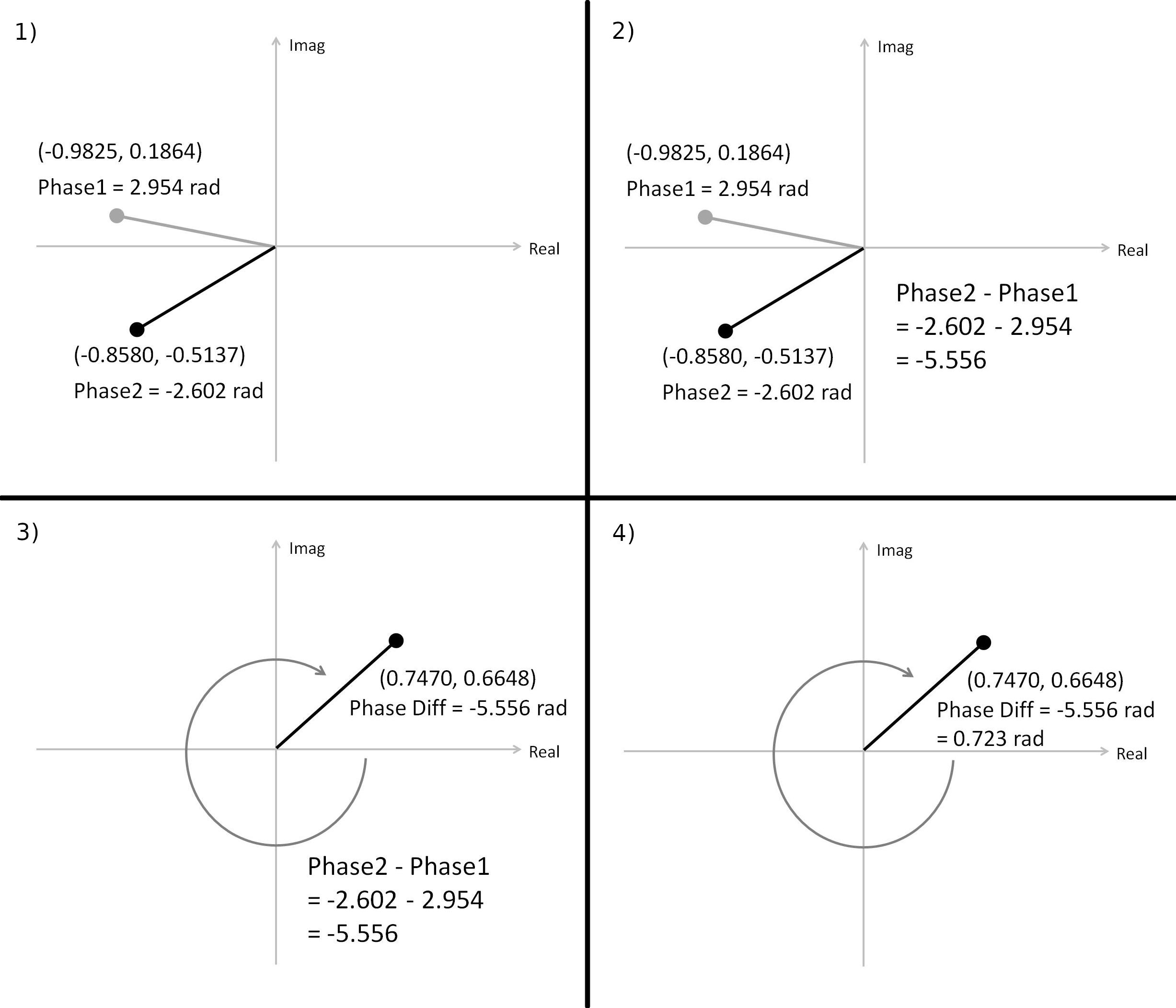
The idea here is this. Rather than calculate the phase difference in polar form, calculate the phase difference in Cartesian form. This can be done by dividing a complex sample by the one that came before it. This will be the same as calculating the phase difference. Except since it is done in Cartesian, rather than polar, form, it will be the "corrected" phase before the actual phase itself is calculated.

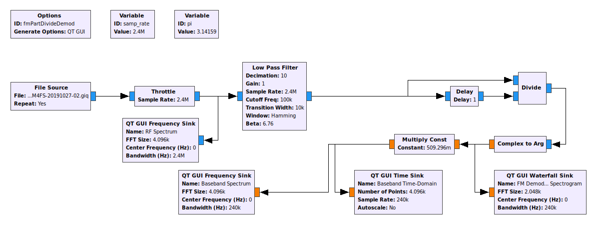
Graph that incorporates division using complex samples in Cartesian form. One sample is delayed, then by dividing its value from the current sample, the quotient a complex sample whose phase is the phase difference between the two samples. Clear as mud? Okay, then, we're walking, we're walking... The only thing left to do is to calculate the actual phase itself ("Complex to Arg" block) and scaling ("Multiply Const" block).

Time-domain and spectral graphs showing output from polar discriminator by dividing consecutive complex samples.

Except computers don't really do division. They do multiplication. Which begs the question, "How can you multiply in order to divide?" The most straightforward way is to multiply by the inverse of a number. Actual inverse operations really only work on floating point numbers. And that's what we're talking about here, anyway. GRC complex samples are actually 32-bit floating point numbers, both for the real and imaginary part. That means that each complex sample requires a total of 64 bits (8 bytes). But that's not the important thing. Floating point numbers exist as a mantissa (the decimal part) and exponent. Want to invert a number that has an exponent? Simple. Flip the sign on the exponent.

Except that's not what we're talking about here. We're talking about dividing one complex sample by another complex sample. The math is a bit different here. Skipping over all of the complexity, if you want to divide one complex sample by another, conjugate the sample in the denominator. That's it. Flip the sign of the imaginary part of the complex sample in the denominator, and VIOLA! It's essentially "inverted" for purposes of multiplication with another complex sample. And that's how most systems do this. They'll take a stream of complex samples, delay-and-conjugate it, then multiply it by the current sample. The delay means it becomes the previous sample (since we're interested in the phase difference between samples) and conjugate it (the "invert" part so that we can use multiplication and not division), then we multiply the two samples (delayed-and-conjugated times the current sample). The output is another complex sample, but this new sample has as its phase the phase difference between the current and previous sample. The multiplication is followed by the "Complex to Arg" block in order to calculate the actual phase difference, followed by a scaling ("Multiply Const" block) to create the final, frequency demodulated output.

Let me just say this straight. This is brilliant. This is what engineers kill for. A workable solution that is elegant and practical. Rather than calculate the phase, then calculate the phase difference, first calculate the phase difference, then calculate the phase. Again, just, plain brilliant.

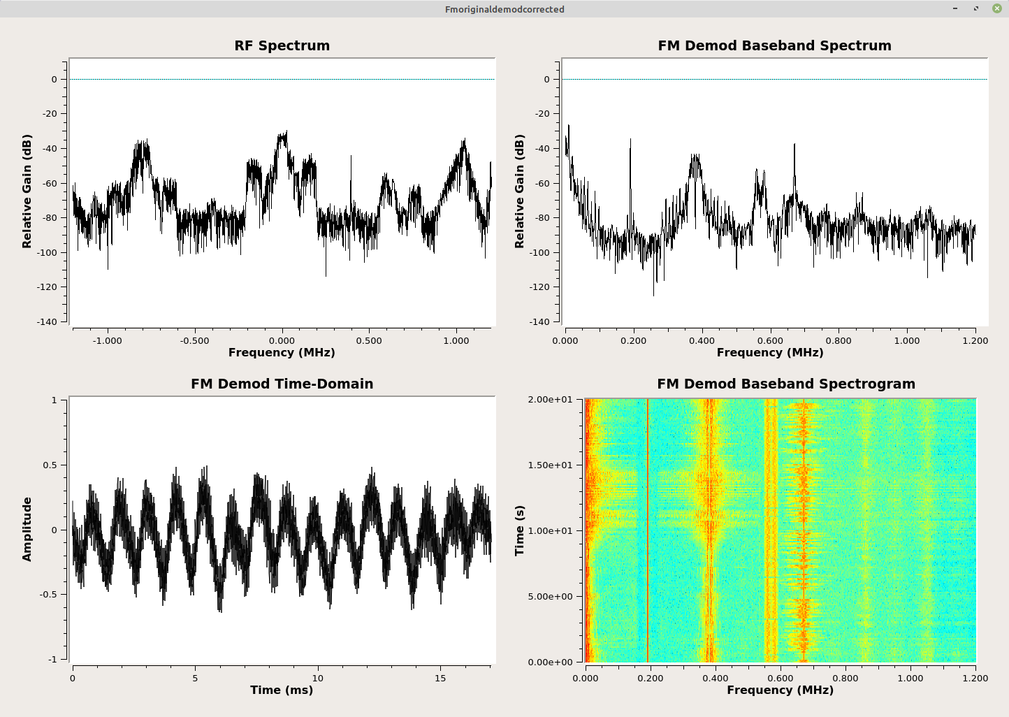
NOTE: This is the math that I got wrong in my previous post. Based on the text documentation of the "Quad Demod" block of GRC, I thought that the current sample was conjugated, and the delayed sample was not. It turns out that still works, but technically the output will be amplitude inverted. The correct one, as explained in Jim Shima's paper from 1995 (and he was not the first to figure this out), is to delay-and-conjugate the same sample, then multiply it with the current sample.

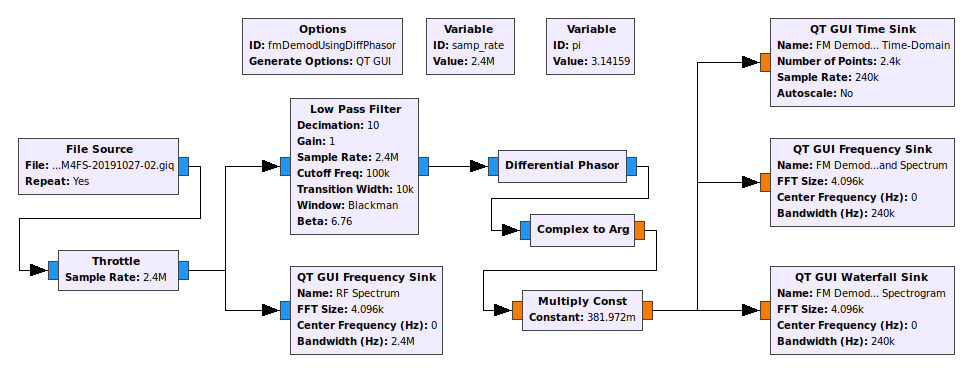
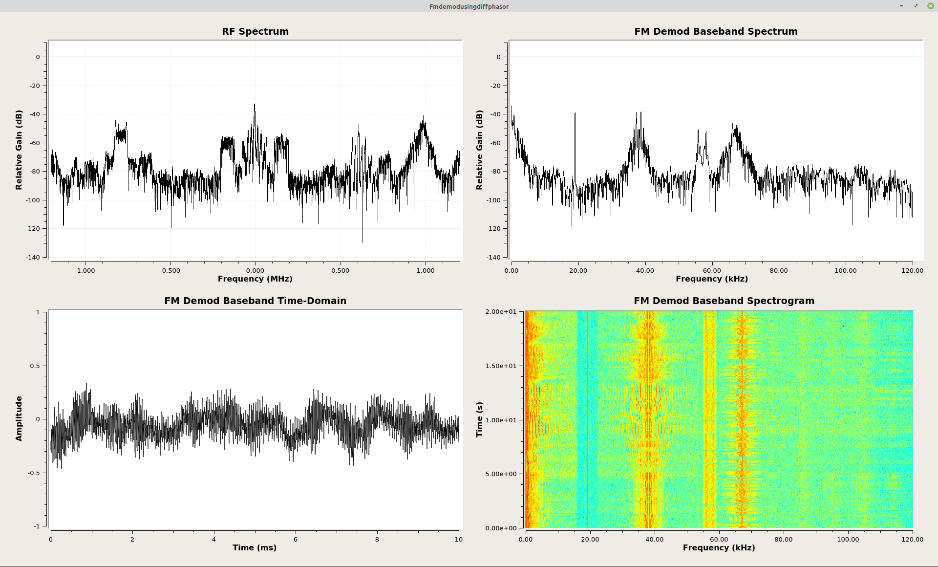
GRC graph showing how to construct a straightforward polar discriminator. One sample from the FM signal is delayed and conjugated, then multiplied with the current sample. The output is fed into a "Complex to Arg" block in order to calculate the phase of the product sample; this phase is the phase difference. Once it is scaled using the "Multiply Const" block, the output is the FM discriminated signal. This set-up is identical to the "Quad Demod" block.

Time-domain and spectral graphs showing the output for the polar discriminator using the delay-and-conjugate multiply method.

The Polar Discriminator - Somewhat Simplified

It turns out that GRC provides the delay-and-conjugate multiply operation in one block. It's called the "Differential Phasor" block. This gives a graph as shown below.

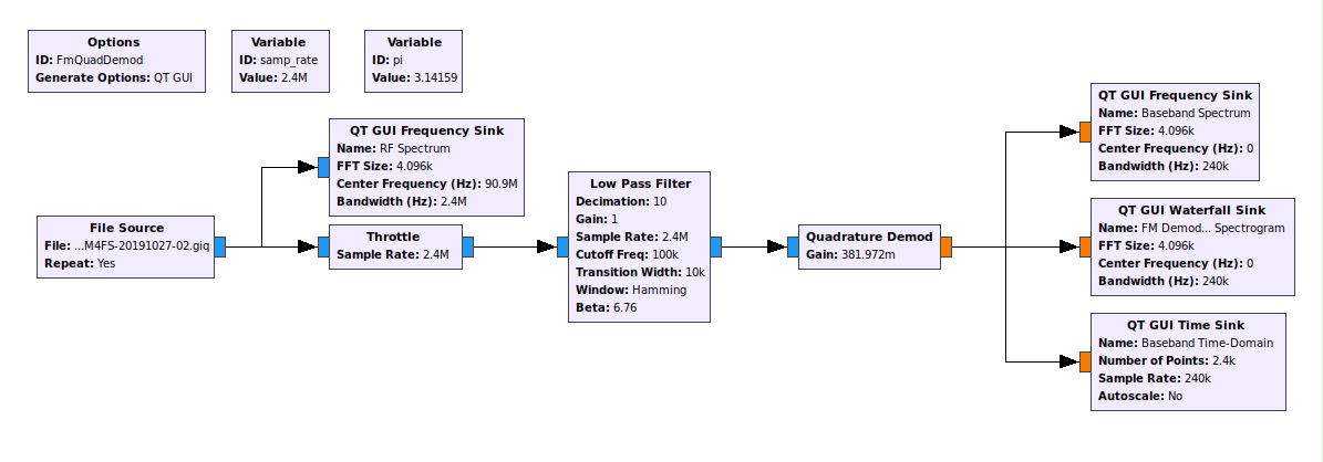
Graph of a polar discriminator, only swapping out the "Delay", "Conjugate", and "Multiply" blocks for the one block "Differential Phasor".

Time-domain and spectral graphs of the output using the "Differential Phasor" block.

The Polar Discriminator - Completely Simplified

The graph for the polar discriminator I outlined above is, well, complicated. Turns out that GRC puts it altogether in one block, the "Quad Demod" block. That block combines the delay-and-conjugate multiply operation, the arctangent function (the "Complex to Arg" block), and the scaling (which in the "Quad Demod" block is called "Gain"), all in one block.

This is the graph using the "Quad Demod" block. This block combines the delay-and-conjugate operation, the multiply operation, the arctangent (aka "arg") operation and scaling operation (which is called the "Gain" in the "Quad Demod" block) all into one block.

Time-domain and spectra for FM discriminator using the "Quad Demod" block.

One of the confusing aspects of the "Quad Demod" block when you first use it is, "What is this 'Gain' setting? How do I set it?" This setting is nothing more than a scaling of the output. FM, again, is the change of phase over time. The two, important parameters here are the sample rate and the number of radians in a circle (2π). If you want the output of the "Quad Demod" block to be "Hz", then you could calculate the "Gain" setting as follows:

\( Gain = {{ Sample Rate } \over { 2 \pi }} \)

You may have noticed that I include a "Variable" block in many of my graphs with the value for "pi". That's why.

But what if you want to push the output of the "Quad Demod" block into an "Audio Sink" block? The above equation won't work. The amplitudes will be waaaaaay too high. The "Audio Sink" block wants samples that are between +/- 1. To make this possible, you need to divide the value above by the frequency deviation of the FM transmitter. For FM broadcast, this is 75 kHz. I add in a little wiggle room for safety purposes. If you want to listen to audio with the "Quad Demod" block, the gain should be as follows:

\( Gain = {{ Sample Rate } \over { 2 \pi \times 100e3 }} \)

The code for the "Gain" setting directly would appear as follows. NOTE: This assumes you have a "Variable" block for "pi", where its value is "3.14159".

samp_rate/(2*pi*100e3)

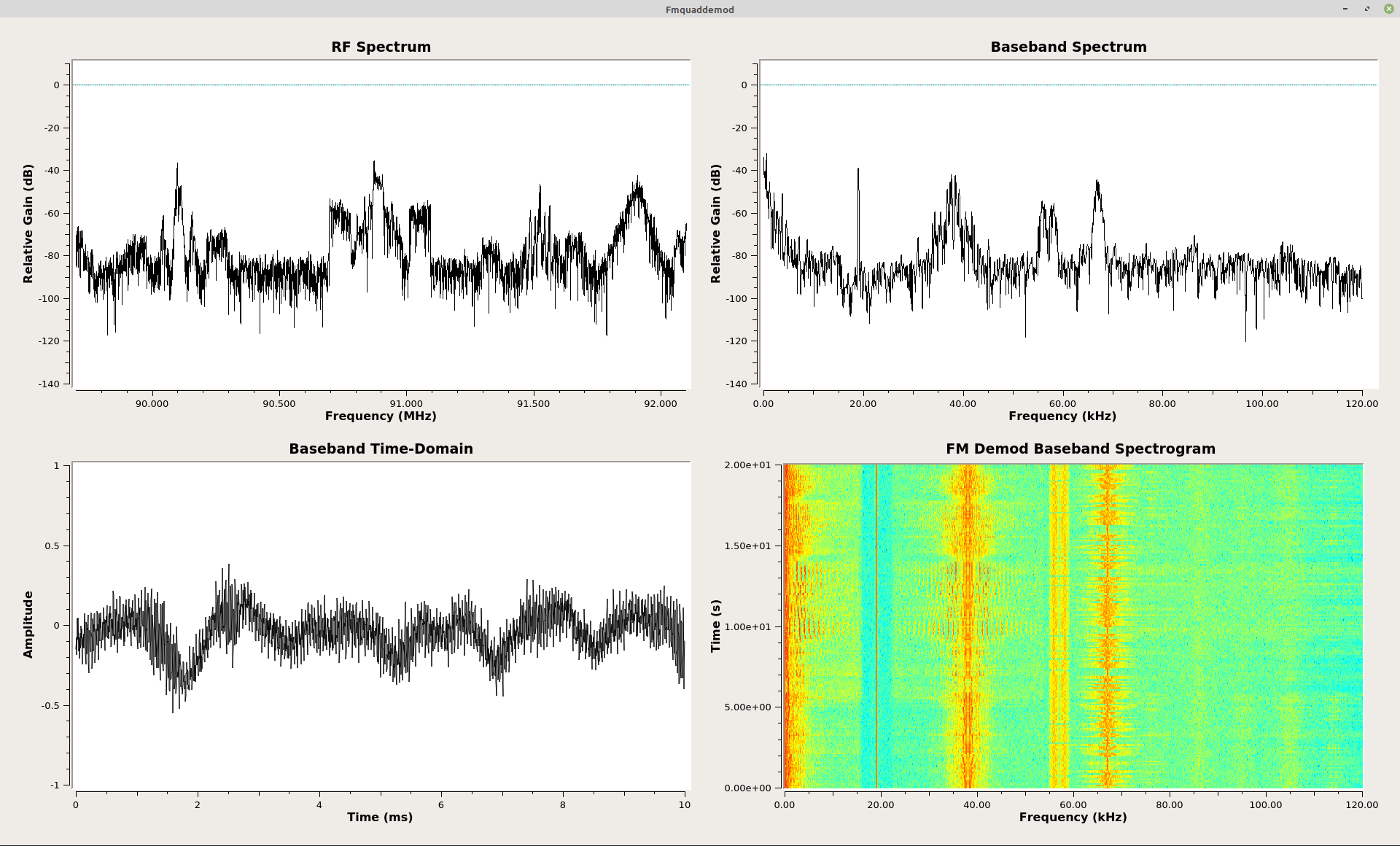
The Polar Discriminator without the Arctangent Function - Take #1

In my previous post, I went through Rick Lyons' method to create a polar discriminator without using the arctangent ("arg") function. It turns out that that function requires a bit o' processing. Here it is, once again, in all of its glory.

This graph is the implementation of Rick Lyons' circuit to implement a polar discriminator, but without using the arctangent function.

Time-domain and spectra of the output of the polar discriminator without using the arctangent function. The most interesting aspect is that the baseband spectra arcs lower in amplitude as it increases in frequency. This is unlike most of the others, which tend to increase in amplitude with higher frequency.

The Polar Discriminator Without the Arctangent Function - Take #2

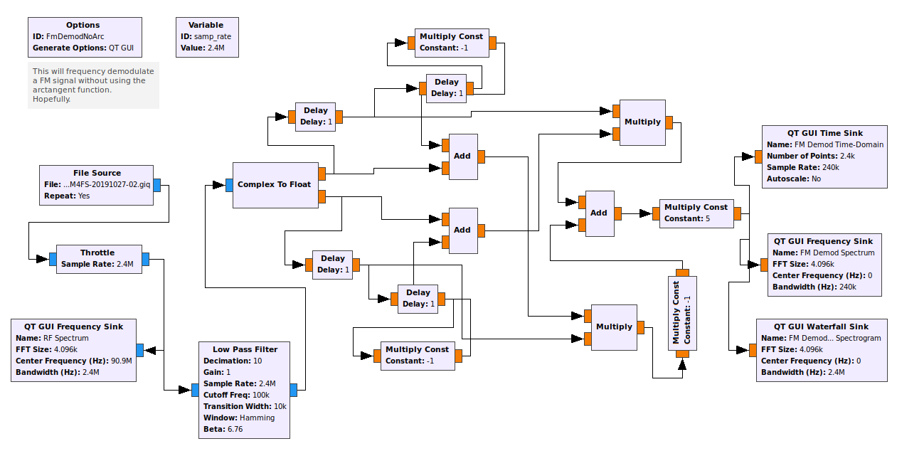
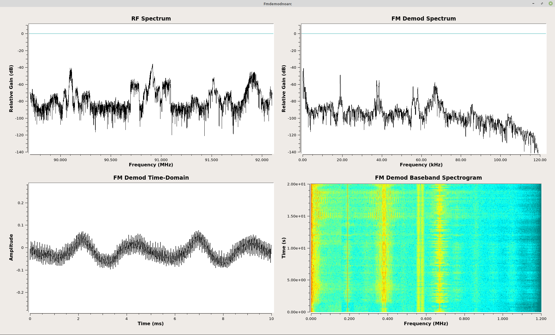
As I was pondering Rick Lyons' frequency demodulator without using the "arctangent" function, I had an epiphany. There's yet one more way to frequency demodulate a signal without the arctangent function. The short answer is this: Run the polar discriminator at a much higher sample rate than Nyquist (typically 6 - 10 times), then simply use the imaginary component at the output of the multiplication of the delayed-&-conjugated sample with the current sample.

I'm not the first one to think of this, either. While looking for information on who developed the delay-&-conjugate method, I found an entry in Google groups that mentions this oversampling method. That entry was posted in October of 1995. I'm at least 24 years late to the party. Typical. Of interest is that one of the people in that Google groups discussion was "Jim Shima", possibly the same one as the thesis discussed above.

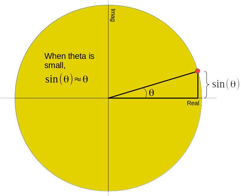
With a high sample rate, the phase of the FM signal will not change much in between samples. The polar discriminator multiplies two complex samples to calculate the phase difference. The product is another complex sample. That final complex sample will have a phase, θ. It turns out that when θ is small, the value of the sin(θ) will be roughly equivalent to θ. Sin(θ) is the same as the imaginary component in the polar plot. So with a relatively high sample rate, we can create a frequency discriminator by multiplying using the delay-&-conjugate method, then taking the imaginary component of the resulting complex sample. No need to perform the arctangent function.

The product of the current complex sample with a delayed-&-conjugated complex sample creates a third complex sample, as seen here. If the sample rate is high, the phase created from that complex sample will be small. This means that the size of the imaginary component will be roughly equal to the angle itself.

Gnu Radio Companion showing receiver for FM broadcast station. The sample rate is kept high all the way through the discriminator. The discriminator consists of the "Differential Phasor" block and the "Complex to Imag" block. The "Differential Phasor" block performs the delay-and-conjugate followed by the multiply operations of a polar discriminator. The "Complex to Imag" block pulls out the imaginary component of each complex sample. With the high sample rate, the phase will not change much between samples. This means that θ ~= sin(θ) = imaginary component, and we've effectively frequency demodulated the FM signal. After the discriminator (at the output of the "Complex to Imag" block), the signal is downsampled.

Gnu Radio Companion time-domain (top) and frequency-domain (bottom) plots from output of frequency demodulator. This shows how the baseband signal appears from the the demodulator using the oversampled imaginary component rather than the arctangent function.

The question becomes, "How high of a sample rate do you need for this to work?" Would you accept, "It depends"? The main thing it depends on is how much error you're willing to tolerate in the output signal. At angles up to roughly 30 degrees, the difference between θ and sin(θ) is less than 5%. That's my limit. The Google groups discussion mentioned angles up to 45 degrees (π/4 radians). That much of an angle provides an error of 10%. If the sample rate is at the Nyquist limit, the maximum phase change between samples will be 180 degrees. To ensure that the maximum phase change is 30 degrees or less (my preference), I would have to sample at 6x over the Nyquist rate. The example I used was a FM broadcast station. It's a 200 kHz bandwidth and requires a 200 kHz complex sample rate. This means I would have to sample at 1.2 MHz minimum to ensure that I stay within these bounds.

Frankly, I do not consider this to be a viable technique. It's more of an interesting phenomenon (said in the way of Leonard Nimoy's Spock). However, the Google groups entry suggests at the end:

Now, not to muddy the water, but for audio FM I have heard of some subjective tests that found users prefering [sic] the compressed audio that results from using the imag approximation for big angles. Is this related to the solid state vs. tube amp debate?

What is the right answer? I'll let you decide.

"Give Me the Easiest FM Receiver!"

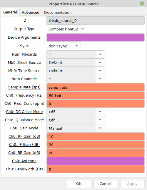
If you wound up on this page because some search engine said, "Hey, check out this web site if you want to make a FM receiver using Gnu Radio Companion!", well, welcome! Without further ado, here's the most straightforward FM receiver for an FM broadcast signal you can create. In my opinion. And here's the GRC file, if you just want to download it. You should be able to right-click on the link and select "Save link as..."

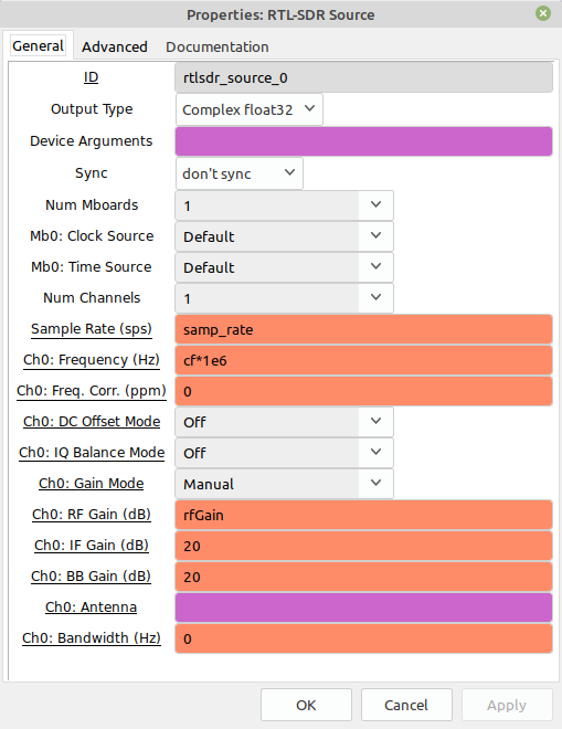
NOTE: This is based on using a RTL-SDR as the source. If you have a different front end (HackRF One, LimeSDR, USRP, whatever), you'll have to substitute the appropriate block for the "RTL-SDR Source" block in the graph below.

Basic FM receiver graph. You'll have to manually set the center frequency, as shown below. This graph assumes you're trying to receive an FM broadcast station.

"Variable" block used to set the overall sample rate. This is the sample rate at the output of the RTL-SDR (or whatever SDR you will use). Once it passes through the "Low Pass Filter" block, the sample rate will be 240 kHz. This is due to the decimation by 10 in the LPF (2.4 MHz / 10 = 240 kHz). Then, at the output of the "WBFM Receive" block, it will be 48 kHz due to the decimation by 5 (240 kHz / 5 = 48 kHz).

"RTL-SDR Source" block settings. If you're **not** using a RTL-SDR, you'll need to change this block and substitute whatever block is appropriate (HackRF, USRP, LimeSDR, whatever). The center frequency, labeled as "Ch0: Frequency (Hz)", is set to 90.9 MHz ("90.9e6"). Set this to whatever you want the center frequency to be.

"Low Pass Filter" block. Note that the "Transition Width" setting drives how much work your processor has to do. The smaller this setting, the more work required. Therefore, if you're running this graph on a low-end processor and you have skipping, one thing you might try is to increase this setting. For example, you could try increasing it to 20 kHz ("20e3").

"WBFM Receive" block. It asks for a confusing setting, "Quadrature Rate". **That's just the sample rate at the input of the block.** Because the input for this graph is 2.4 MHz, which is then decimated by 10 (in the "Low Pass Filter" block), the sample rate (aka "Quadrature Rate") is 2.4 MHz / 10 = 240 kHz. Audio cards want specific sample rates. My audio card will take 48 kHz. That's why I selected 2.4 MHz. When I decimate it by 10, the output sample rate of 240 kHz is more than enough to handle the FM signal (bandwidth of 200 kHz). When I then decimate *that* by a factor of 5, 240 kHz / 5 = 48 kHz.

"Audio Sink" block. All you should have to do here is select "48 kHz" from the dropdown menu.

The Basic Receiver with a Few Extras

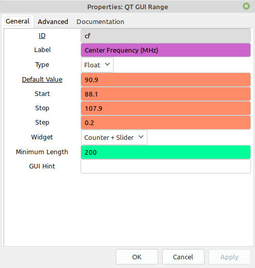
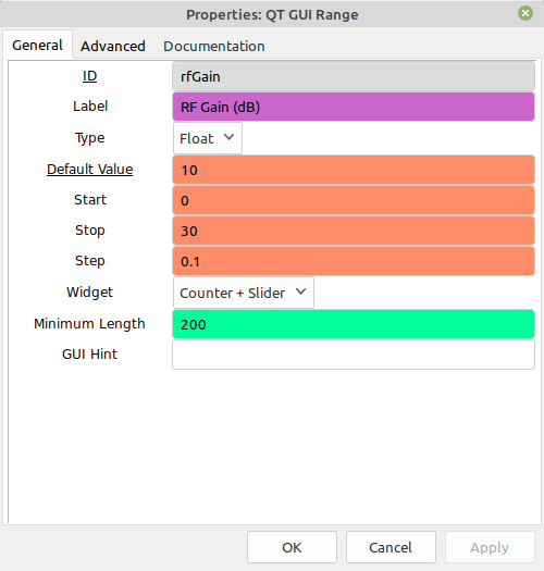
Here's the same receiver, but with an added frequency and gain adjustment widgets. This makes it easier to set the center frequency and gain while the graph is running. Again, the GRC file if you just want to download it.

Graph of a basic FM receiver for the FM broadcast band. The values and settings for each of the boxes are listed below.

"QT GUI Frequency Sink" block settings. NOTE: This block is optional. If you want to make your graph even simpler (and just want to listen to the audio), leave it out. I like to have it as a "sanity check" that my graph is working properly.

"QT GUI Range" block used to set the center frequency of the receiver. This block is also optional. If you don't want to use it, put the frequency directly into the "Ch0: Frequency (Hz)" setting in the "RTL-SDR Source" block. For example, if your favorite station is 94.7, then directly enter that into the "Ch0: Frequency (Hz)" setting as "94.7e6". Also, these frequencies are for US stations (88 - 108 MHz, in 200 kHz increments, with the center at odd values starting at 0.1). If you're in a foreign country, you'll have to set this range and step size to whatever values work for you.

"QT GUI Range" block used to set the RF gain of the RTL-SDR. The RTL-SDR only has one gain option, and that is the "RF Gain". The other, two options listed in the "RTL-SDR Source" block ("IF Gain" and "BB Gain") do not apply to the RTL-SDR, and changing those values has no affect on the RTL-SDR operation. This is another optional block. If you leave this out and do not change the default setting, most likely your RTL-SDR will work just fine. At my house, however, I'm roughly 1.5 km from a FM broadcast tower, with another about 3 km away. Between these two, they can overdrive my RTL-SDR if I do not lower the RF gain from its default setting. YMMV.

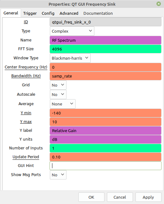
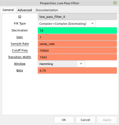
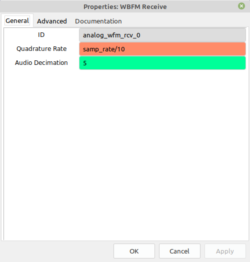
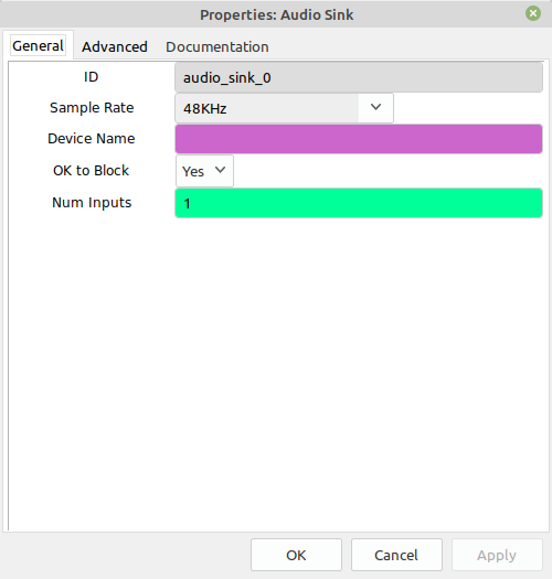
That's pretty much it. The graph above takes the input RF spectrum, filters out all but the desired signal (the one centered in the spectrum if you're using the "QT GUI Frequency Sink" block), FM discriminates it (aka "frequency demodulates it"), filters it some more, then sends these demodulated and filtered samples to the audio sink. If everything is working correctly, you'll hear the audio from the broadcast FM station.

Random Quote Board