Creating a Variable RBW Spectral Display in Gnu Radio

Gary Schafer, April 2023

I've talked about spectral displays before (and again a few months later). I even included a short blurb on how Spike created variable resolution bandwidths. For this post, I'm going to walk through how to build a spectral display in Gnu Radio that let's you set the resolution bandwidth to pretty much whatever you want. This is contrast to most (all?) SDR programs which only allow you to use RBWs that are based on the power-of-2 record length used to calculate the FFT.

Assuming a fixed sample rate, the general order to create a variable RBW is as follows:

Calculate the length, Nd, of the time record needed for the desired RBW.
Collect samples into a time record of length Nd.
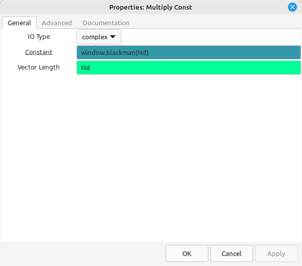
Window the time record.
Zeropad the data so that its length, N, is a power-of-2.
Calculate the FFT.
Calculate the magnitudes of each spectral point.
Display the spectrum.

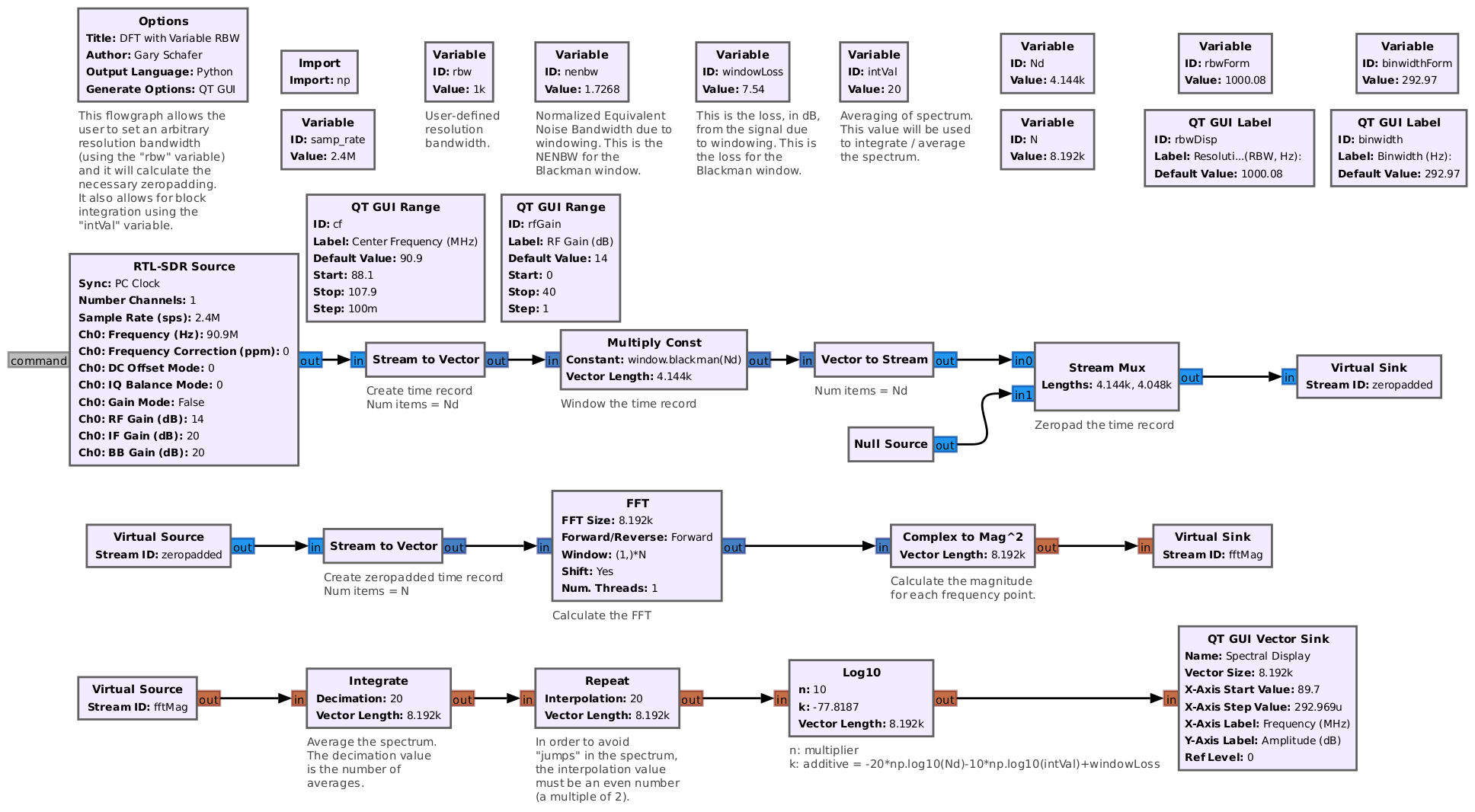
The general flowgraph is shown below.

Gnu Radio Companion flowgraph for variable RBW spectral display. There are four variables that you need to enter data into. These are the "rbw" block, the "nenbw" block, the "windowLoss" block, and the "intVal" block. All others are calculated for you. Unlike the large time record FFT graph from my previous post, this time, the windowing and FFT blocks are separate. This is due to the fact that we have to collect the data, window it, THEN zeropad it before sending the time record to the FFT block. After that, it's a matter of averaging (the "Integrate" and "Repeat" blocks), followed by the "Log10" block (set the amplitudes to a dB scale), then display the information.

Enter the User Variables

This flowgraph requires the user to enter several variables. These are:

Desired RBW ("rbw"): The system will attempt to create a RBW as close to this value as possible. NOTE: It will almost certainly not be precisely this value; it should be close enough.
NENBW ("nenbw"): To calculate the RBW precisely, the system will need to know the normalized equivalent noise bandwidth (NENBW) of the window used. I've included a short table below with the values of several windows available in Gnu Radio.
Window Loss ("windowLoss"): This accounts for the fact that windowing the time record attenuates / removes part of the signal. This value is only necessary if you're concerned about having (roughly) accurate amplitude values. Otherwise, set it to "1".
Integration Value ("intVal"): This is the number of spectra to average together. This will lower the variance of the signals and noise and make it look smoother.

Table 1: NENBW Values
Window	NENBW
Rectangular	1.000
Hanning	1.500
Hamming	1.363
Blackman	1.727
Blackman-harris	2.004
Flattop	3.770

Calculating the Time Record Lengths

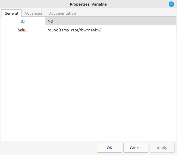
With a known sample rate (f_s), desired RBW, and the NENBW, it's possible to calculate the length of the time record, Nd.

Nd = round(NENBW*f_s/RBW)

The "round" function ensures that the result is an integer.

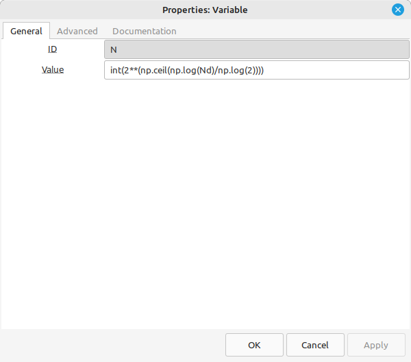
Next, the graph calculates the required power-of-2 length of the final time record after zeropadding.

N = int(2**(np.ceil(np.log(Nd)/np.log(2))))

This calculates the value for Nd as a power-of-2. Then it rounds up. The result is entered as an exponent for 2^X. This is the value used to calculate the final time record length, which must be a power-of-2 in order to be entered into the FFT block.

NOTE: Because of the two functions, "np.ceil" and "np.log", the flowgraph must also have an "Import" block with the value "import numpy as np".

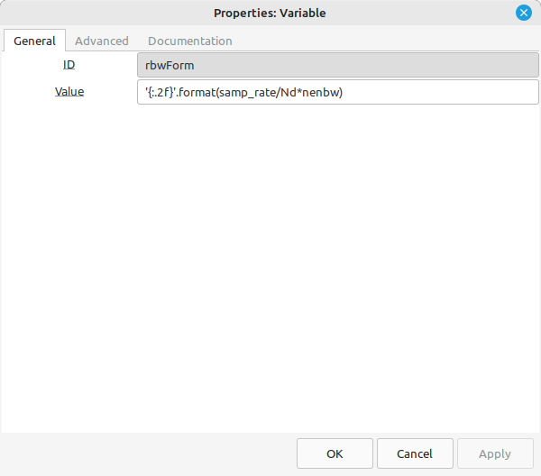
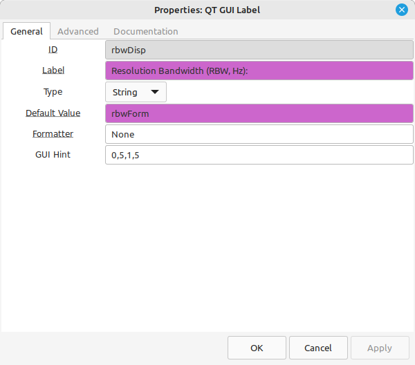
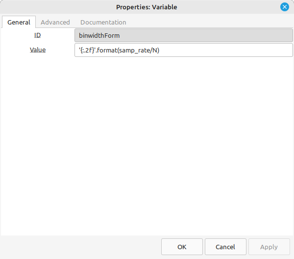
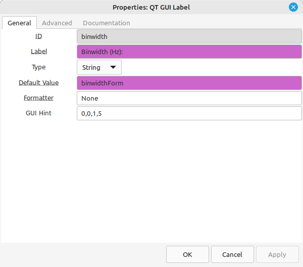
"Variable" block used to calculate the length of the data time record based on the desired RBW.

"Variable" block used to calculate the power-of-2 time record length, N.

Calculate and Display Actual RBW and Binwidth

Because of the rounding required to calculate Nd (it must be an integer, after all), the actual RBW value will be slightly different than desired.

RBW_actual = f_s*NENBW/Nd

Binwidth = f_s/N

"Variable" block that calculates and formats the actual RBW.

"Label" block used to display the actual RBW.

"Variable" block that calculates and formats the binwidth of the spectral display.

"Label" block used to display the binwidth of the spectral display.

Walking Through the Flowgraph

This flowgraph will work just fine with either a file source (combined with a "Throttle" block) as well as with a SDR source. For this example, I'm using a RTL-SDR.

The output of the samples (SDR, file) is sent to a "Stream to Vector" block. This collects Nd samples and sends it on to the "Multiply Const" block. The "Multiply Const" block performs the actual windowing.

Properties for the first "Vector to Stream" block.

"Multiply Const" block used for windowing the time record.

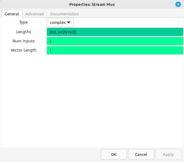
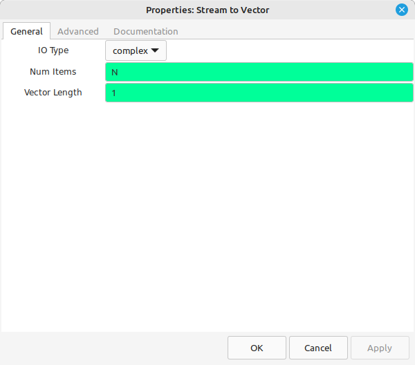
The next step is to zeropad the time record so that the time record length is a power-of-2. This has to be performed as individual samples (hence, the "Vector to Stream" block). The "Stream Mux" block first pulls in Nd samples, followed by N-Nd samples as zeros (from the "Null Source"). The last step is to turn the stream back into a vector.

"Stream Mux" block. It first pulls in Nd samples of data, then N-Nd zeros as the zeropadding.

Second "Stream to Vector" block. This creates the final, zeropadded time record that will be sent to the FFT.

FFT block. The "Window" entry is set to all 1s (equivalent to a "Rectangular" window) since the windowing was performed already.

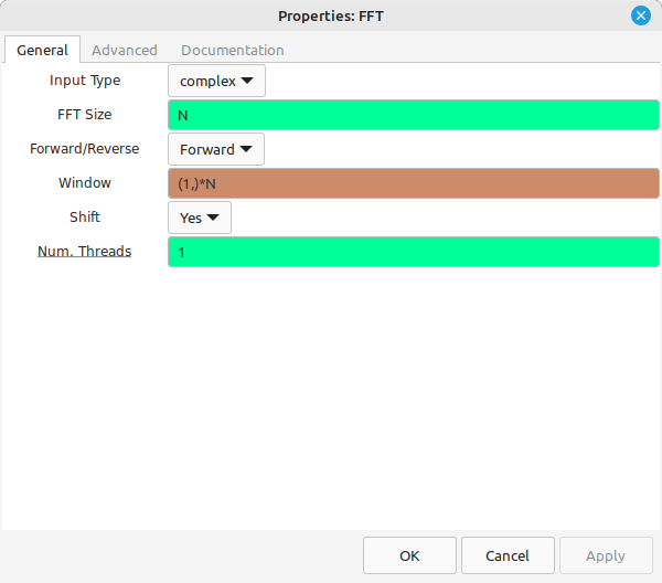
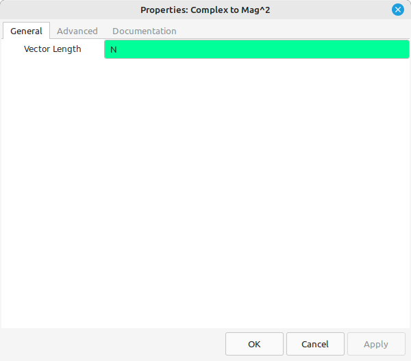
The step after the FFT is to calculate the magnitudes of each point. The last step will be equivalent to a 20log₁₀ calculation. Rather than using "20", we can simplify the magnitude calculation by setting it to "Complex to Mag^2". This avoids having to calculate the square root (a costly process), and only means that the "Log10" block requires a value of "10" for "n".

"Complex to Mag^2" block. This calculates the magnitudes of each spectral point.

The "Integrate" and "Repeat" blocks form the averaging circuit.

"Repeat" block used to flush the cache. This block also stops the "jumps" in the spectrum seen if this block is left out of the flowgraph. (NOTE: No idea why those jumps occur, but it's due to the zeropadding.

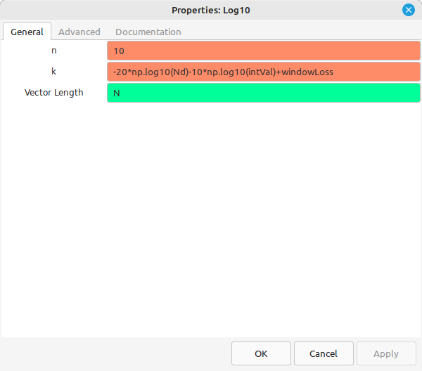
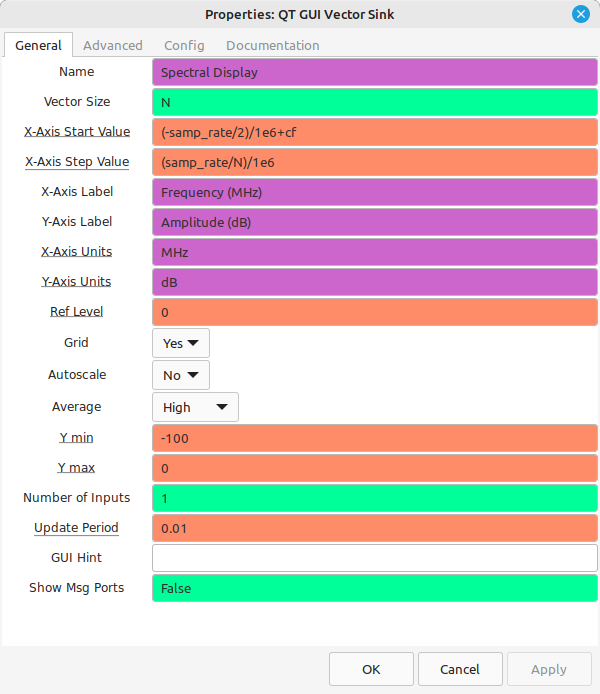
The second-to-last block converts the magnitudes to a logarithmic scale, adjust the magnitudes for differences due to the length of the data time record (Nd), the length of the FFT and the window loss. The final block creates the actual display of the spectral data.

"Log10" block. This converts the magnitudes essentially to a dB (decibel) scale. It also adjusts magnitudes to account for the length of the data time record (Nd), the length of the FFT (N), and window loss.

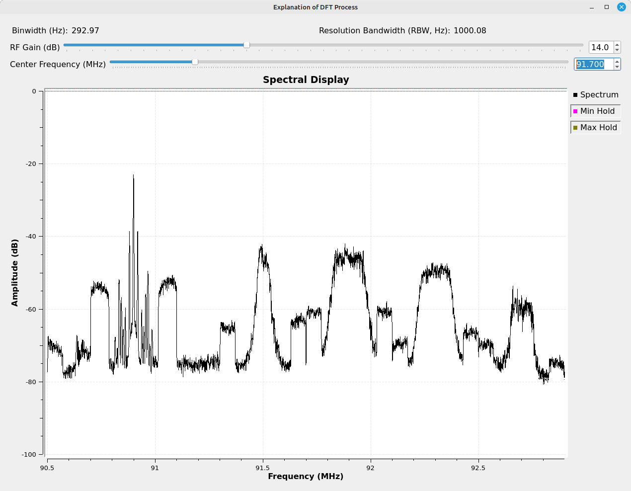
"Vector Sink" block used to display the spectral data. The horizontal axis has been adjusted so that its values are in MHz. The vertical scale is a relative dB value.

The final result is a spectral display that can have a wide range of resolution bandwidths.

Final spectrum from a RTL-SDR centered at 91.7 MHz with a 2.4 MHz sample rate, a desired RBW of 1.0 kHz, and 20 averages.

Random Quote Board

Creating a Variable RBW Spectral Display in Gnu Radio

Enter the User Variables

Calculating the Time Record Lengths

Calculate and Display Actual RBW and Binwidth

Walking Through the Flowgraph

Here's a Random Fact...