Gnu Radio and Narrow Resolution Frequency Displays

Gary Schafer, June 2021

I love graphs. Spectral displays are perhaps my favorite form of art. Weird? Perhaps. But here we are. Gnu Radio provides the two, basic signal analysis graphs, time domain (aka "oscilloscope") and frequency domain (aka "spectrum analyzer"). The current versions of Gnu Radio provide two, basic displays for spectral information. These are the "QT GUI Frequency Sink" and the "QT GUI Waterfall Sink". The only issue with these displays is that they are limited in the number of samples they can process at one time. For some reason, the "QT GUI Frequency Sink" is limited to one sample less than 2¹⁴ (16383). I find that strange. One more and it would be possible to perform an FFT of 16384, or precisely 2¹⁴ samples.

Anyway, if you want to create narrow resolution spectral displays, your options are:

Use a low sample rate (and low bandwidth). This is the basis of the "zoom FFT". This method only provides narrow resolution within a narrow bandwidth. The general steps are to frequency shift the desire part of the spectrum to near 0 Hz, filter the signal, lower the sample rate (decimate), then calculate and display the FFT.
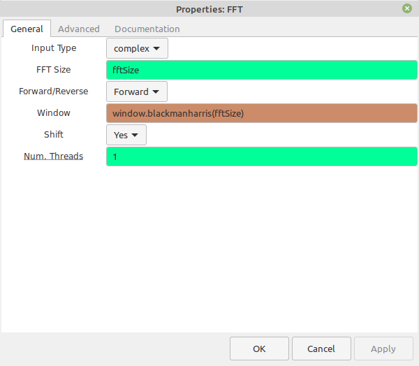
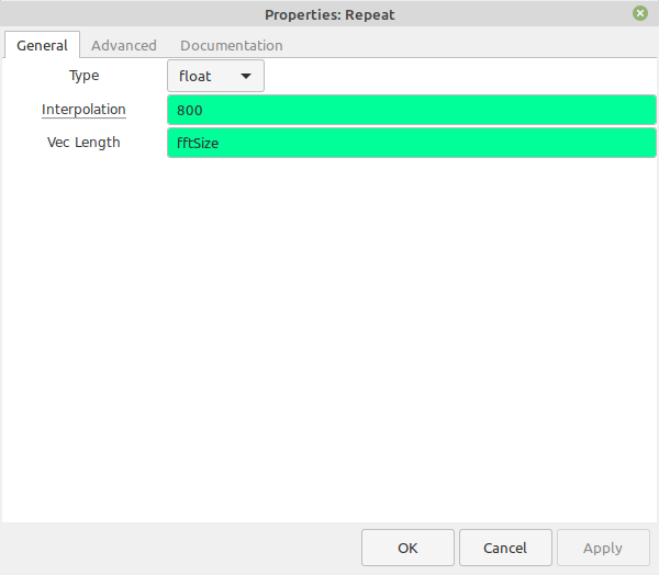
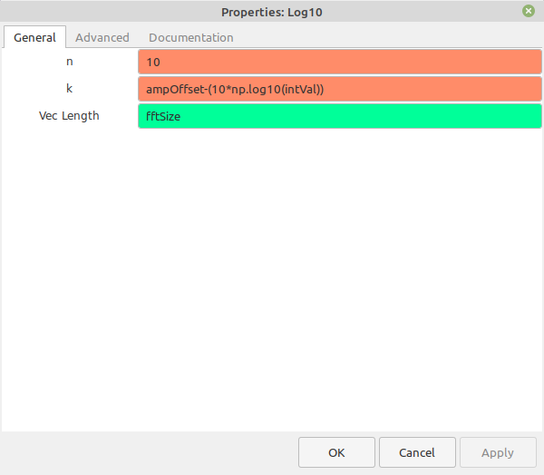
Build your own FFT displays. Gnu Radio provides the basic block diagram in their wiki article on the FFT block. The big issue here, as stated in the article, is that you have to calculate the magnitudes and frequency scales manually. However, if you really want to understand how a FFT display works, I think this is it.

Zoom FFT

The basic idea of the zoom FFT is summed up in the equation for calculating resolution bandwidth.

RBW = β * f_S / N

Given a certain window (β) and a fixed number of samples in the time record (N), the resolution bandwidth is directly related to the sample rate. The zoom FFT is based on the idea that if we can reduce the sample rate, we can reduce the resolution bandwidth.

Reducing the sample rate means decimation, which means filtering to avoid aliasing the signal. A very basic setup would be as follows:

A basic setup for a zoom FFT display would be a lowpass filter coming off of the source and a decimation before the frequency sink. The source is a RTL-SDR. Such SDRs require a minimum sample rate of 900 kHz. However, I've discovered that anything less than 1.1 MHz does not work well.

We can add a basic frequency shifter, then use that to dial the narrow band filter over the larger spectrum.

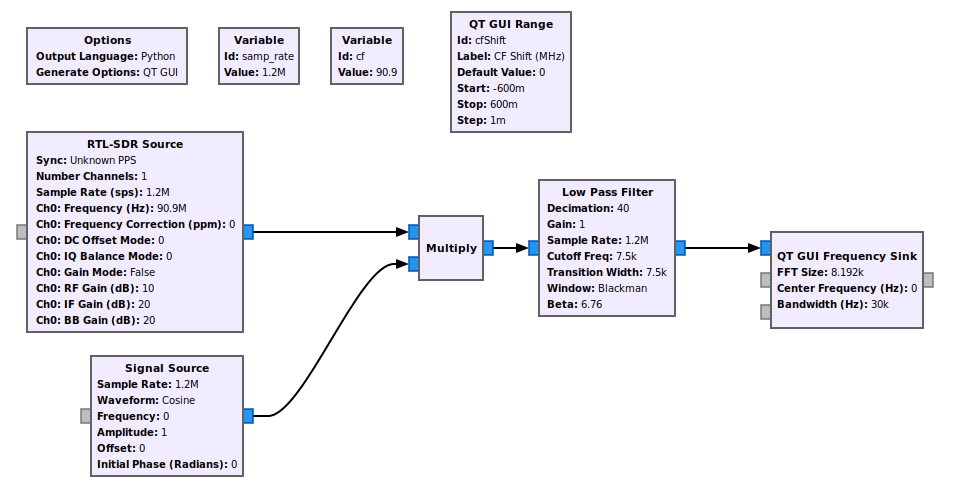
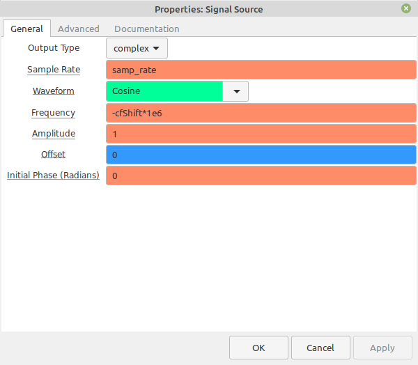
This is the zoom FFT with a frequency shift. This does not change the center frequency of the SDR. It changes the portion of the spectrum which will be zoomed.

This is the properties for the "Signal Source" block. The frequency is set to negative (-) so that the change of the frequency corresponds with the portion of the spectrum that will be covered.

I've added a bit more bling with the addition of a second frequency sink that will show where the zoom FFT is focused.

This is the same as the previous graph, with the addition of a second bandpass filter and frequency sink. The bandpass filter uses complex taps so that it can be focused on a single portion of the original spectrum. If the filter used real taps, it would have to use two, different portions of the spectrum that were the same frequency from the center (mirror images).

These are the properties for the bandpass filter using complex, not real ("float"), taps.

Large Time Record FFT

The other way we can reduce the resolution bandwidth is by increasing the number of samples in the time record. This means increasing the "N" value from the equation above.

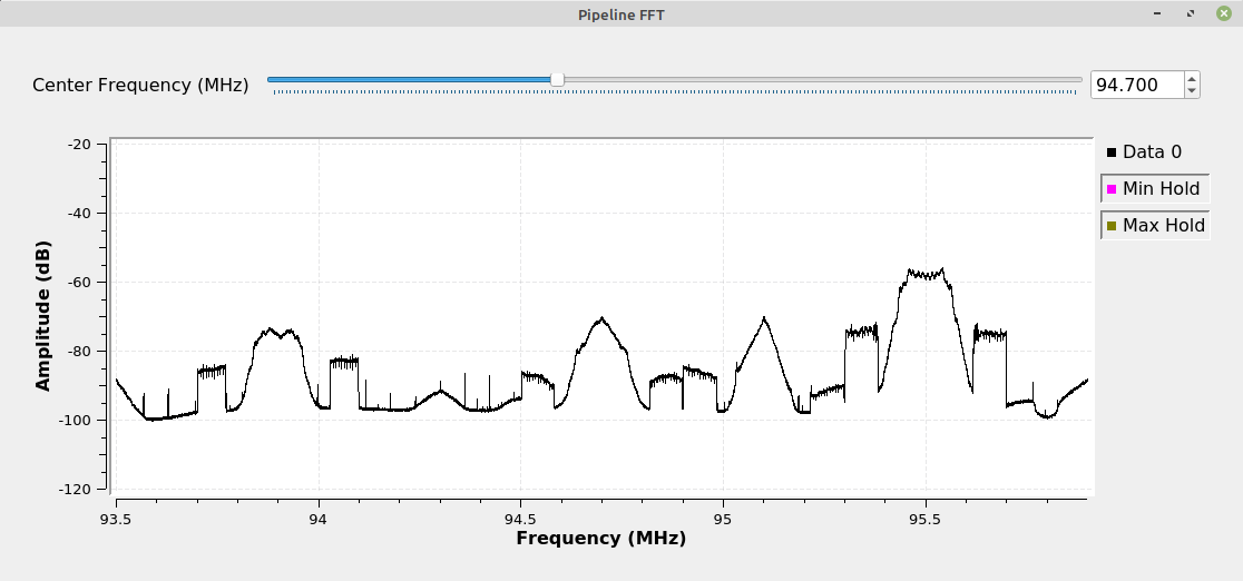
As stated before, the current versions of Gnu Radio only allow for the "QT GUI Frequency Sink", and that display is limited to 2¹⁴-1 (16383) samples. If you want more samples than this, you'll need to create your own frequency display. While the Gnu Radio wiki provides such a graph, Paul Boven at the Dwingeloo Radio Observatory provided a more interesting graph that adds averaging.

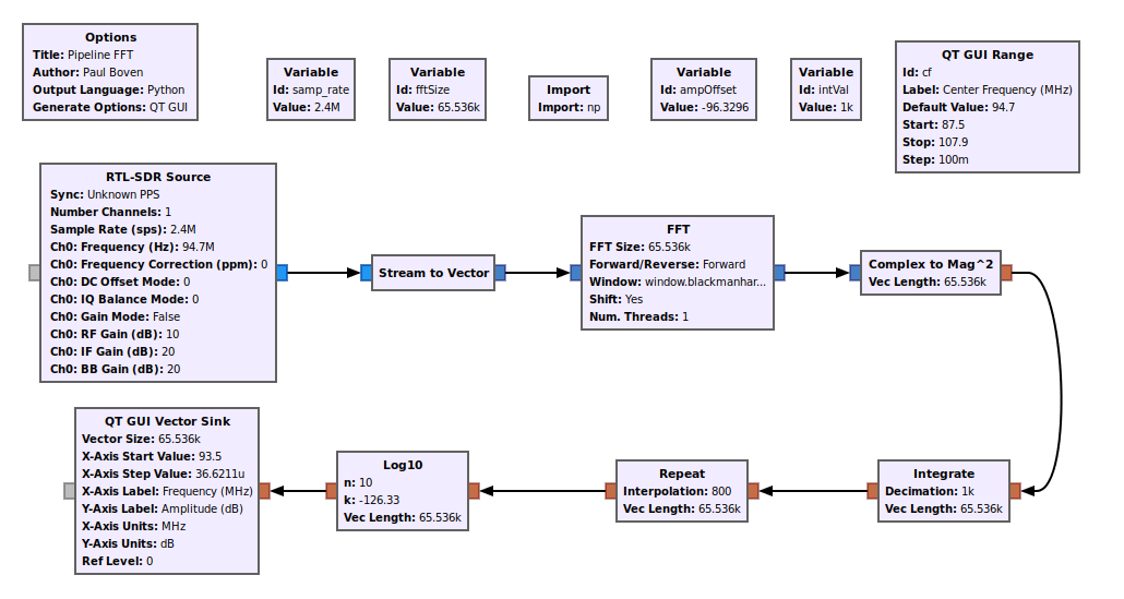
Graph of the large sample value FFT with averaging.

Paul and his astronomical cohorts look for radio signals from distant stars. I tend to have more terrestrial uses, such as being able to look at the FM broadcast band with narrow resolutions and, thus, being able to see the number of frequency partitions in the IBOC channels.

Here's the thing about this graph. The graph will integrate (add up) 1000 (or whatever value you place in the variable "intVal") FFTs, and with each FFT (on this graph) calculating 65,536 samples, that's a total of (65536)(1000) = 65.5 million samples. With a sample rate of 2.4 MHz, this means it will take (65.5e6)/(2.4e6) = 27.3 seconds between updates. You can reduce this rate either by lowering the size of the FFT, or by reducing the number of integrations.

This is a spectrum of 2.4 MHz using a 65k sample FFT. The FFT uses the Blackman window, which means a window factor of roughly 2. The RBW is thus roughly (2.4 MHz)*(2)/(65536) = 73 Hz. The spectrum also shows various spikes, probably based on intermodulation within the RF tuner chip.

This is the same spectrum (RBW ~= 73 Hz) but zoomed in on one of the IBOC sidebands. This clearly shows the frequency partitions of the IBOC signal. Each frequency partition is a OFDM signal made up of 19 subcarriers. Each subcarrier is roughly 363 Hz wide, while each partition is roughly 6.9 kHz wide.

Random Quote Board

Gnu Radio and Narrow Resolution Frequency Displays

Zoom FFT

Large Time Record FFT

Here's a Random Fact...