Creating a FFT Filter with Gnu Radio Companion

Gary Schafer, October 2025

Acknowledgement: This post would not have been possible without Steven W. Smith's book, "The Scientist and Engineer's Guide to Digital Signal Processing. While Dr. Smith has made his book available for download for free, please support such great work by buying a hardcopy from your favorite book vendor.

There are two ways to filter a signal. One is in the time domain; the other is in the frequency domain. Either way, you're convolving the input signal with the filter impulse response. The time domain requires a lot multiplies and adds. Every sample has to be multiplied with every tap of the filter. Thus, if we have a 201 tap filter, then passing 201 samples through the filter would require 201² multiplies, since each sample is multiplied by each tap in the filter. (NOTE: There's also the adds requiring 201 adds for each sample, thus the filter has to do 201² multiplies and 201² adds for each 201 samples.) Let's just say that that is a lot.

That's in the time domain. In the frequency domain, it's different. Convolution in the time domain is equivalent to multiplication in the frequency domain.

Time domain convolution is equivalent to frequency domain multiplication. — Time domain convolution is equivalent to multiplication in the frequency domain.

The reason that this equivalency is a really good thing can be summed up in three words: fast Fourier transform. The FFT is the super-efficient version of the discrete Fourier transform (DFT). The FFT requires many fewer calculations than would otherwise be the case. The equivalency of "convolution in time domain = multiplication in the frequency domain" plus the efficiency of the FFT combined means we can create digital filters that require much less processing than would otherwise be the case.

Speed Test of Time vs FFT Filter in GRC

From a user standpoint in Gnu Radio Companion, there's no difference between the time domain and frequency domain filters. They're straightforward blocks. For either case, we add the block to the flowgraph, adjust the parameters, and away we go.

But, from a processing standpoint, there's a big difference. I'm going to make a straightforward flowgraph to show the difference.

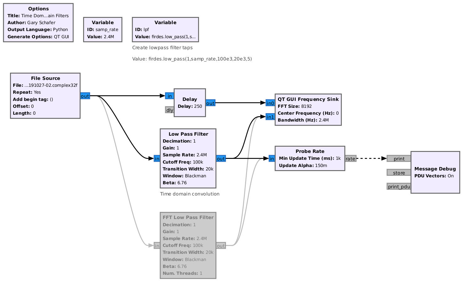
Block diagram showing several blocks connected from left to right. The blocks are entitled, from left to right, file source, throttle, low pass filter, and frequency sink. — Gnu Radio flowgraph used to compare the speed differences for the time domain (top block, entitled "Low Pass Filter") and the frequency domain (bottom block, "FFT Low Pass Filter"). The output of the block passes into a "Probe Rate" block. The "Message Debug" block prints the output of the "Probe Rate" block to the terminal in Gnu Radio. The "FFT Low Pass Filter" is currently disabled. When testing this specific block, it is enabled and the "Low Pass Filter" is disabled.

Running this flowgraph, we're not really interested in the display. Rather, we're interested in the terminal in the lower, lefthand corner. The messages for the "Low Pass Filter" (time domain convolution) appeared as follows:

******* MESSAGE DEBUG PRINT ********
(((rate_now . 2.55393e+07) (rate_avg . 2.55992e+07)))
************************************

The maximum sample rate on my system for this time domain filter and parameters (2.4 MHz sample rate, 20 kHz transition width, Blackman window) is roughly 25.6 MSam/sec. Switching over to the "FFT Low Pass Filter" (frequency domain convolution), I get the following message:

******* MESSAGE DEBUG PRINT ********
(((rate_now . 3.25155e+08) (rate_avg . 3.24794e+08)))
************************************

With the frequency domain convolution, the speed has increased to roughly 325 MSam/sec. On my primary desktop computer, the frequency domain convolution is over 12 times faster than the time domain convolution. This speed test is dependent on the number of taps in the filter (fewer taps may mean the time domain is faster), the computer system (CPU, motherboard, RAM, and because I'm reading from the hard drive, drive read speed), operating system, and the specific version of Gnu Radio I'm using. But the general idea is valid.

Running this same flowgraph on a slower machine (i5-5200U vs the i9-13900 of my main computer), the time domain convolution is 7.45 MSam/sec, while the frequency domain convolution is 59.3 MSam/sec. This is only roughly 8 times faster. But its still significantly faster.

FFT Filter in GRC

How does this work? What are the steps for creating such a filter? Let's start with a general block diagram.

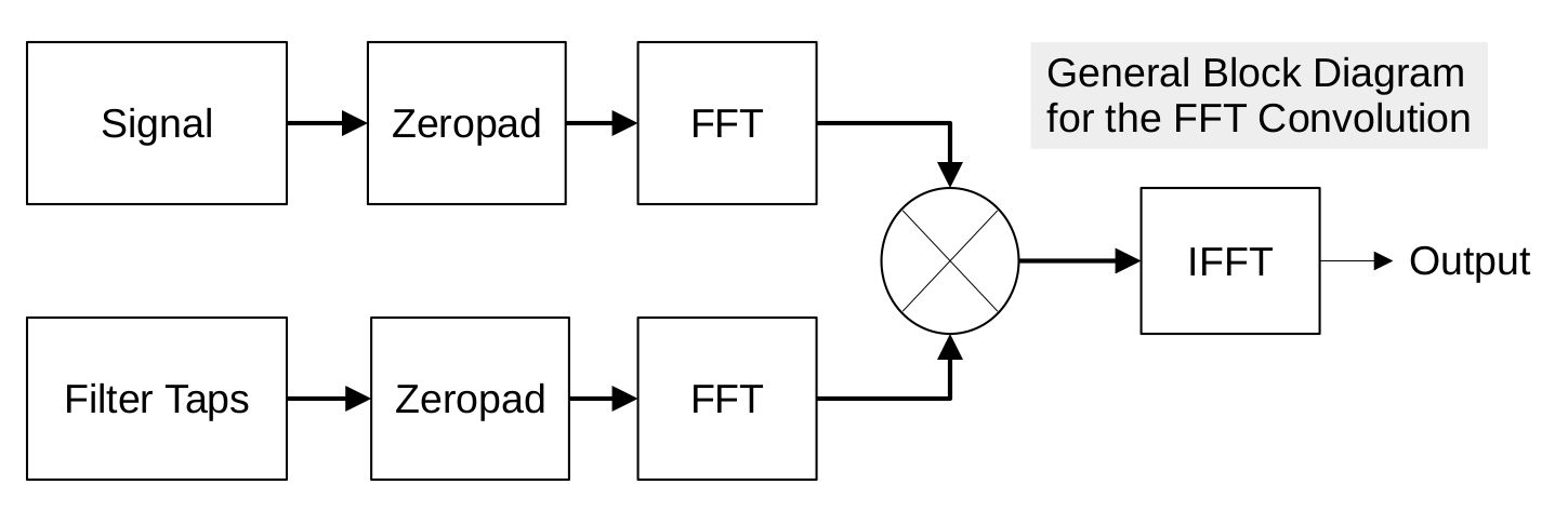
General block diagram for performing convolution in the frequency domain. Both the signal and filter taps are zeropadded, then converted to the frequency domain with the FFT, multiplied together, then the signal is converted back to the time domain.

Where did the zeropadding come from? Let's continue the discussion with that.

FFT Convolution and Zeropadding

The FFT is a block-oriented algorithm. It does not work on a sample-by-sample basis; it works on a block of samples all at the same time. The algorithm takes in a block of samples (which, depending on which description you're reading may be called an array, a vector, or a time record) representing the time domain and outputs a block of samples representing the frequency domain. The important point here is that the size of the two blocks (input time domain and output frequency domain) are the same size.

The question becomes, "How big does this block of input points need to be?" The one part that has very little adjustment is the number of filter taps. Gnu Radio uses the harris approximation to calculate the number of taps. While this is an approximation, it gives us a good idea of the number of taps required based on the sample rate, transition width, and attenuation of the window used.

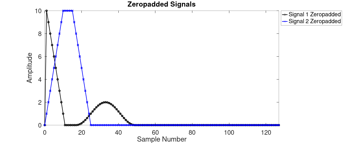
The other question is, "How many signal samples do I need?" The answer is, "How many do you want?" That's right. Put in as many as you want. You can go with fewer samples per block (means more FFT blocks), or more samples per block (means fewer blocks, but more calculations per block). Just for the sake of moving things along, let's assume that we're going to use the same number of signal samples as filter taps. 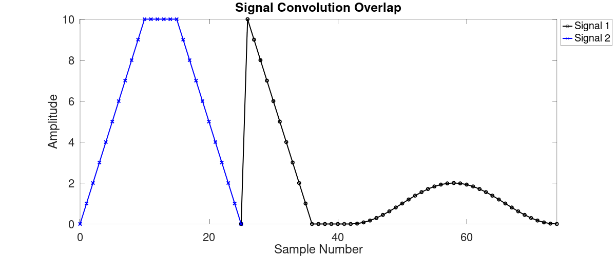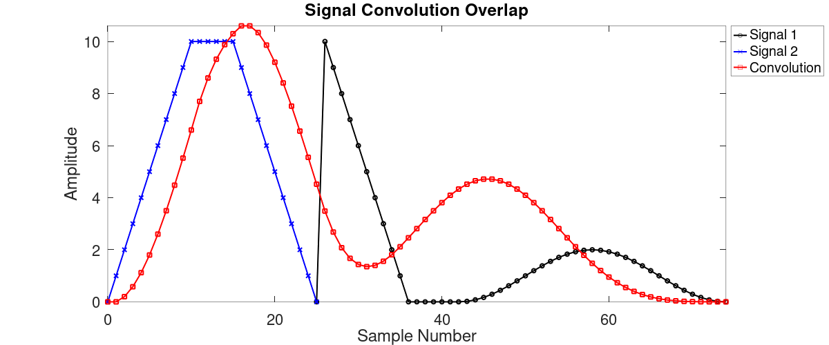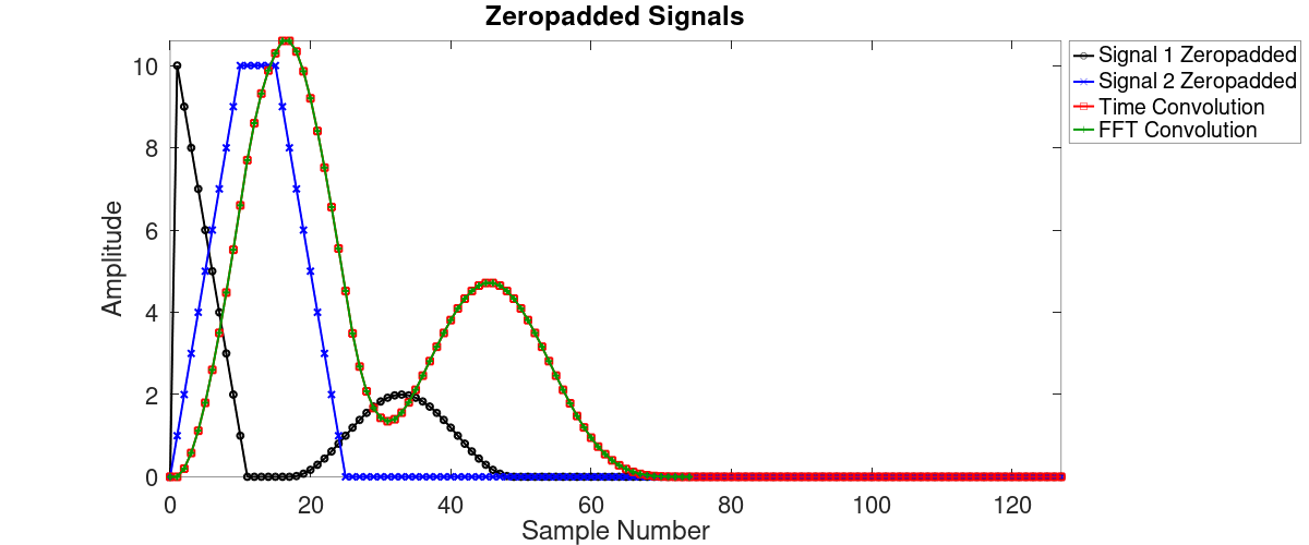And let's say that our "harris approximation" says we need 101 taps. This means we're also going to use 101 signal samples.

Next question: How many samples do we need to feed into the FFT? How large will the block be? We said 101 taps and 101 samples. The output will be the response of the signal convolved with the filter. This effectively spreads out the signal in time. The length of the signal will be spread out in time by the length of the filter. That's a total of 202 points going into the FFT, right? Not quite. The maximum length of the two waveforms (filter and signal) occurs just as they come together. But the response doesn't start until they overlap at one point. When the filter starts, the first tap of the filter covers the first sample of the signal. The maximum size is (filter taps) + (signal samples) - (the one point they have in common). Given these parameters (101 filter taps, 101 signal samples), the maximum size is a convolution output of 201 points. This is the maximum size we need to worry about.

Graph showing two curves. The first curve is blue and is shaped like a triangle with the top cut off. The second curve is black and starts with a narrow peak, flattens out towards the right, and then is half of a sinusoid. — Time domain graph showing two waveforms at the beginning of calculating the convolution. The first signal (black) is 50 samples long; the second signal (blue) is 26 samples long. The total number of points is the length of each signal (26 + 50 points) *minus the one point they have in common*. The total length is 26 + 50 - 1 = 75 points.

Graph showing three curves. The first curve is blue and is shaped like a triangle with the top cut off. The second curve is black and starts with a narrow peak, flattens out towards the right, and then is half of a sinusoid. The third curve is red and extends from one end of the graph to the other. It is shaped like a tall, rounded peak followed by a smaller, somewhat flatter rounded peak on the right end of the graph. — Graph showing the convolution overlaid with the original, two graphs. Note that the convolution is the length of the two original signals combined (minus the one point that they have in common). Consider the convolution to be one of the signals (pick one!) and spread out due to the other signal.

Except the two blocks, filter taps and signal samples, aren't put together and fed into a single FFT. They're separate, and each has to feed into its own FFT. Once the two are multiplied together in the frequency domain, the inverse FFT will be the convolution of the two blocks (filter taps and signal samples). The output block has to account for the spreading of the signal in time. Thus, the overall block size has to be at least equal to the (taps)+(signal)-1. How do we make up the difference for each block? Zeros. We add zeros so that each block (filter and signal) is equal in length to taps + samples -1. We're going to start with the filter taps or signal samples, then we're going to add enough zeros to each so that our output is at least equal to taps+signal-1.

The practical aspect is that we don't just add enough zeros to get us to taps+signal-1. We add this plus enough zeros to get us to a block size that is a power of 2. This makes it easy to feed into the FFT. The next power-of-2 value from 75 is 128.

For our example, we're going to take our filter taps and signal samples and zeropad each to get each block to 128 samples. Thus:

Signal 1 will be zeropadded with 128 - 50 = 78 zeros.
Signal 2 will be zeropadded with 128 - 26 = 102 zeros.

Graph showing two waveforms, both covering from left to right. The first is a black waveform that starts at 0, jumps to the peak, then drops back down to 0 over several points. It stays at 0 for a few points, rises in a shallow curve over many points, then drops back down to 0 roughly halfway across. It stays at 0 over the rest of the graph. The second waveform, in blue, starts at 0, increase to the peak over several points, stays at the peak over several points, then drops back down to 0 over several points. It also stays at 0 over the rest of the graph. — Both waveforms with zeropadding. Each waveform has been extended to 128 points.

Graph showing four waveforms, all of them covering from left to right. The first is a black waveform that starts at 0, jumps to the peak, then drops back down to 0 over several points. It stays at 0 for a few points, rises in a shallow curve over many points, then drops back down to 0 roughly halfway across. It stays at 0 over the rest of the graph. The second waveform, in blue, starts at 0, increase to the peak over several points, stays at the peak over several points, then drops back down to 0 over several points. It also stays at 0 over the rest of the graph. The third one, in red, slowly rises from the left at 0, rises to a relatively narrow, rounded peak, drops back down to a low level, rises up to another rounded peak at roughly halfway up, then drops down to 0 where it stays for the rest of the graph. The fourth one, in green, traces the exact, same path as the third one. — Comparison of two waveforms, both of them zeropadded, with the convolution of these two, zeropadded waveforms. There are two convolutions, one in time and the other using the FFT. The time-domain one is from the original waveforms (non-zeropadded). Note that, even though the time domain one is shorter than the frequency domain one, both of these convolution waveforms are identical.

A Basic GRC Implementation of FFT Convolution

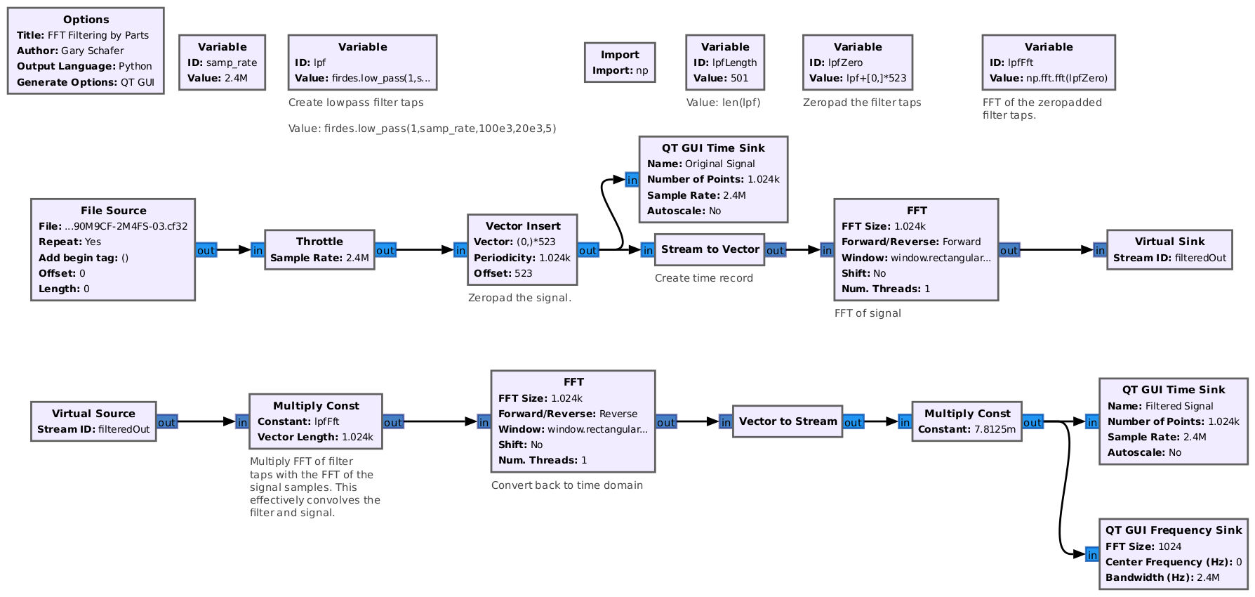
Let's take a look at how this would be implemented. I've created a basic Gnu Radio Companion flowgraph that will filter a set of complex samples (2.4 MHz of the FM broadcast band, centered on a FM station). I'm specifically going to filter out the center station. I'm using the following specifications for the filter:

Cutoff frequency: 100 kHz
Transition width: 20 kHz
Window type: Blackman-harris (attenuation of 92 dB)
Filter taps based on harris approximation: 501
Signal samples: 501 (same as the filter taps)
Size of FFT: 1001 points (501+501-1) -> 1024 points (next power-of-2)
Zeropadding required: 1024 - 501 = 523 zeros

Here's the nice thing about the FFT convolution. Once you have the filter taps, you can pre-calculate the FFT of those taps and store those in memory. You do not have to continually calculate the FFT of the filter taps the same way you do with the signal samples. This reduces the amount of computations required for this convolution implementation. That's what I did with this flowgraph. Rather than using the "FFT" block to calculate the FFT for the filter taps, I'm going to use "Variable" blocks to create the filter taps, zeropad the filter taps, and calculate the FFT of the zeropadded taps using a "numpy" statement.

Speaking of FFT, there's one, key point I should point out. Do not window the data before calculating the FFT. Windowing is used when you're performing spectral analysis, not spectral processing. I set the window in the FFT of the flowgraph to window.rectangular(1024) (or whatever number of points you're sending to the FFT if not 1024). The rectangular window is equivalent to no window.

Block diagram showing a signal flow through various blocks. There are three rows of blocks. The top row consists of setup blocks for various variables. The next two rows perform the actual processing. — Gnu Radio flowgraph to perform a FFT convolution on a signal. The input signal is 2.4 MHz of a FM broadcast band centered on a FM station. The filter is a lowpass filter. The top row of blocks create the filter taps (the variable "lpf"), zeropad the filter taps (the variable "lpfZero"), then calculate the FFT of the zeropadded filter taps (the variable "lpfFft"). The signal passes through the "Vector Insert" block, which zeropads the signal so that it consists of 501 signal samples and 523 zeros for a total of 1024 points. The "Stream to Vector" creates the block (a time record) of 1024 samples. This passes into the FFT block, which converts the time domain samples into the frequency domain. Note that the window is a rectangular window, which is the equivalent of no window. NOTE: You do not want to window the data before calculating the FFT. Windowing is when you're performing *spectral analysis*, not *spectral processing*. It's the next block, the "Multiply Const" block, that multiplies the frequency domain samples of the signal with the pre-calculated frequency domain of the filter taps. This is equivalent to the convolution. The next block is the inverse FFT (IFFT) to convert to the time domain.

Three rows of graphs, with one graph in each row. The top graph shows a series of noisy sinewaves covering the left half of the graph, and a flat line on the right half. The second row is a series of two roughly sinusoidal waves that are less noisy, but now they occupy the center half of the graph. The graph is flat on each end. The bottom graph has a rounded curve in the center occupying roughly 1/10th of the width of the graph. The rest of the graph is empty. — Display of the signal as it is processed. The top most graph is the time domain of the zeropadded signal. The signal occupies the first 501 samples of the display; the rest are zeros added after inputting the signal. The center graph is the time domain of the signal after coming out of the inverse FFT block. It's now been filtered (note that it appears less noisy), but also notice that is has been shifted by roughly 250 samples. This is due to the delay inherent in filtering. The delay is equal to one-half of the number of taps in the FIR filter. Since the filter has 501 taps, the delay is roughly equal to 250 taps. Also note that the signal extends both before and after the signal. This is the filter response, and must be accounted for. This is why the signal must be zeropadded before calculating the FFT of the signal. The last (bottom) graph is the frequency domain plot of the signal. This has been calculated using a rectangular window since, as seen in the middle graph, the signal is "naturally" windowed.

The Signal Gap Problem with the FFT Convolution

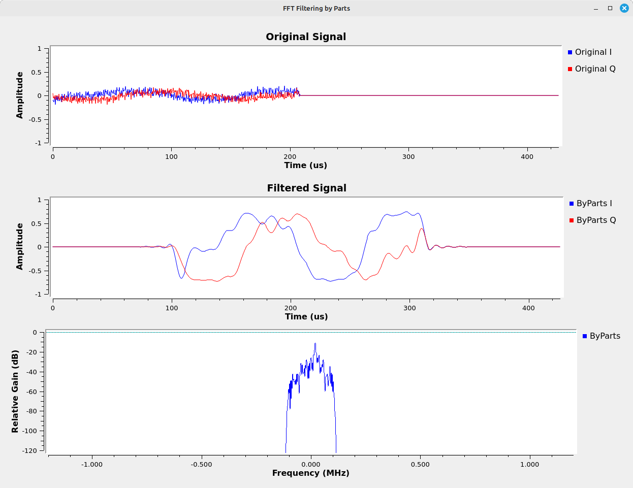
Here's the problem with this simple implementation. Yes, the signal is filtered. But notice that there are gaps in the signal. Look at the center graph above. Yes, it's filtered, but there are gaps of 523 samples between the filtered samples. Let's try a simple way to remove the gaps. I'll modify the flowgraph so that it extracts those filtered samples, and deletes the rest.

Block diagram showing three rows of blocks. The top row is used for setting up various variables. The next, two rows perform signal processing. — Gnu Radio flowgraph that processes a signal using FFT convolution, then extracts the filtered samples and discards the zeropadding. This flowgraph is similar to the previous one, except it adds a parallel path for the "FFT Filter" block (used for comparison purposes), and it adds a "Keep M in N" block to extract the filtered samples and discard the rest.

Three rows of graphs, with a single graph in each row. The top graph shows a signal that is being turned on and off four times along its length. The on times have a roughly sinusoidal appearance. The off times are flat line. The center graph shows two roughly overlapping sinusoidal signals but with small points showing up along its length. The bottom graph shows a roughly long, somewhat flat triangular signal. The signal peaks at the center. The sides are smooth, but the peak has a somewhat noise-like appearance. — This is the display output of the flowgraph. The top graph is at the output of the inverse FFT and shows the filtered signal along with the zeropadding. The "Keep M in N" block extracts the filtered samples and removes the zeropadding. The resulting signal is shown in the center graph. It shows the filtered signal overlaid with the signal as filtered with a standard "FFT Filter" block. Note that there appear to be a few discrepancies in the signal. The FFT of the filtered signal is shown at bottom. Note how it has a relatively shallow set of sidelobes on each side of the signal.

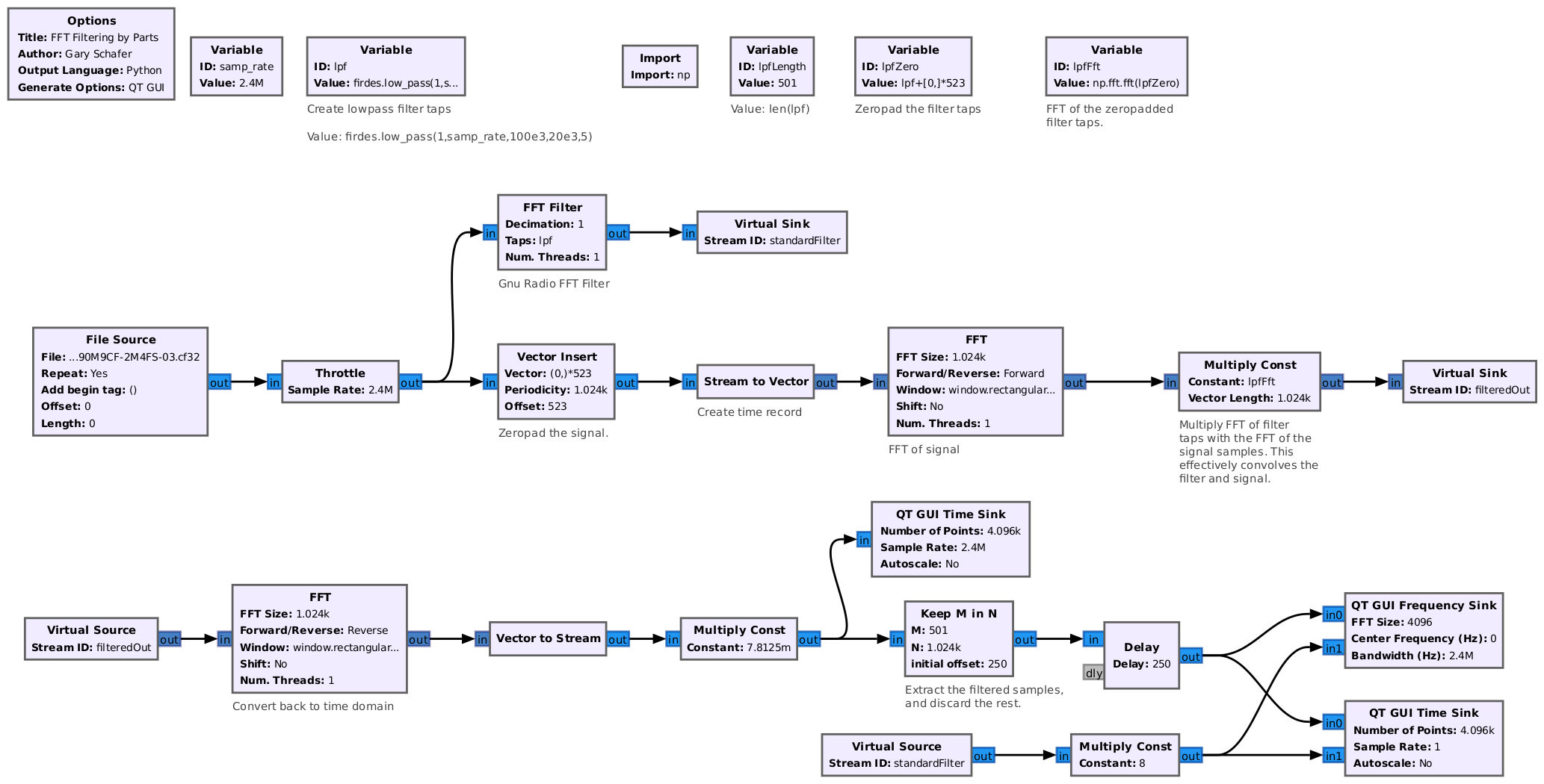
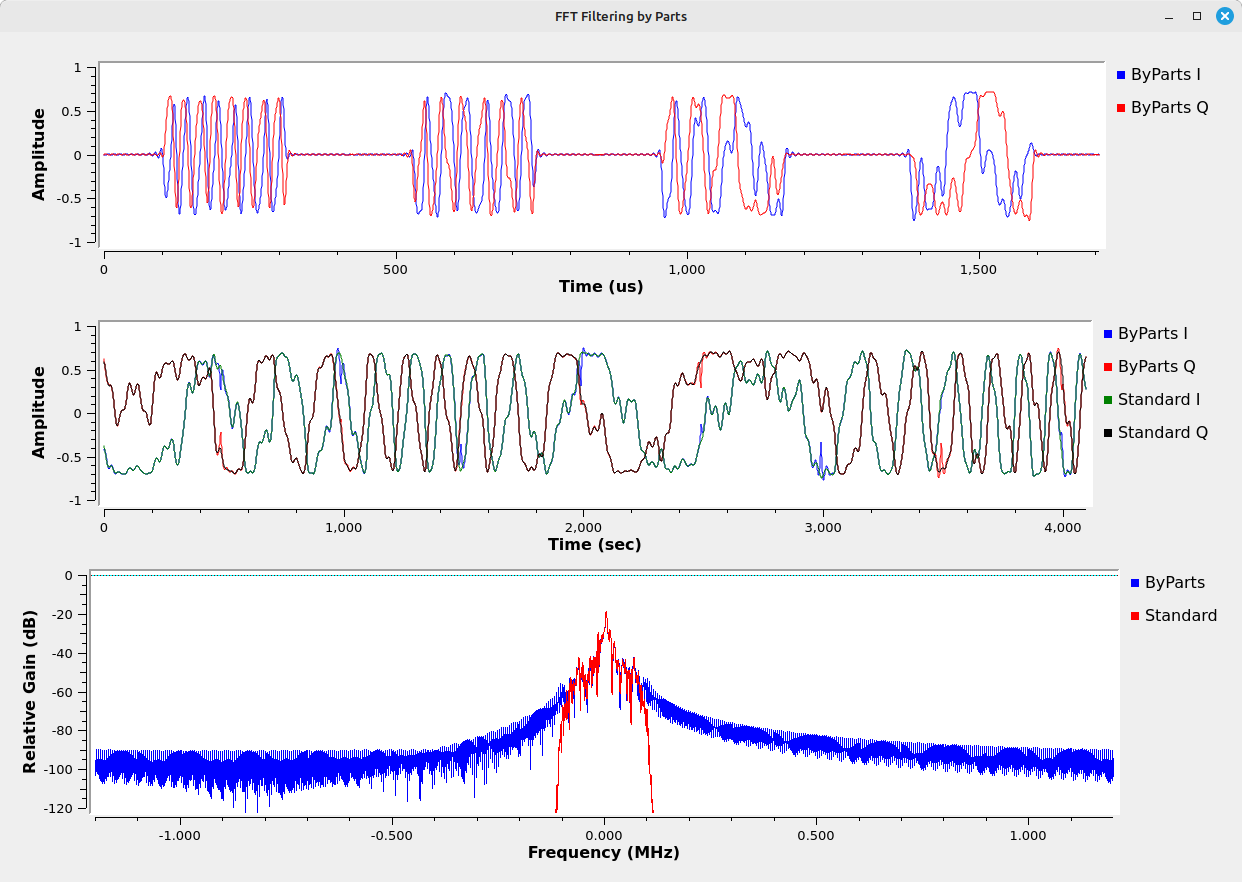
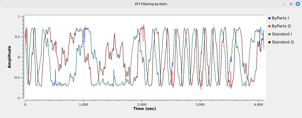
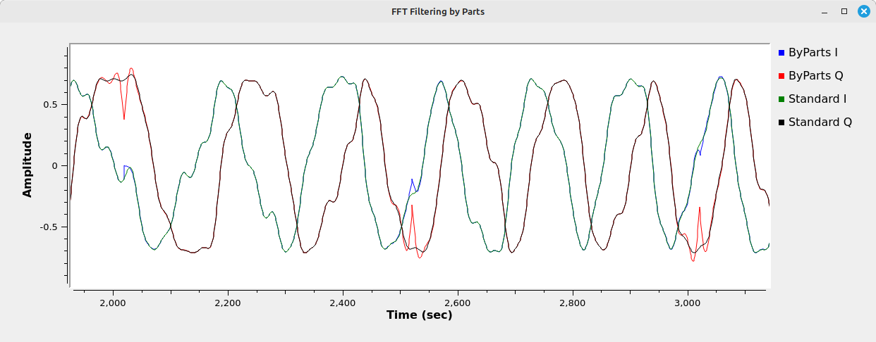
Yes, we've removed the zeropadding, but the signal is still not correct. Look at the frequency domain (bottom graph above). The red shows how the signal should look (it's from the standard "FFT Filter" block), but the blue is how it does look. The noise floor is much higher than it should be. If you look at the time domain graph of the filtered waveform (center graph above), you can see why. Let's zoom in on that waveform to get a better look.

Graph showing two overlaid waveforms that are roughly sinusoidal. One of the sinusoids has occasional peaks appearing on it. — This is a time domain graph showing the FFT convolution overlaid with the filtering using the standard "FFT Filter" block in GRC. Note the presence of small red and blue peaks along the waveform. This is where the signal is going from one 501 point block to another.

Zoomed in view of the time domain graph of the filtered signal. Note the sharp, red peaks. These denote where blocks are stitched together. These also act as impulses which cause a huge jump in the noise floor. It's because of these impulses that the frequency domain display above has such a high noise floor.

Overlap-and-Add Implementation

How do we get rid of those discontinuities? The answer is overlap and add. In other words, do not extract the samples from the filtered blocks. Instead, align the samples so that the end of the samples from one block line up with the beginning samples of the next block. Through the "magic of math" (No, it's not actually magic.), those impulses go away and you wind up with a perfectly continuous waveform. Gnu Radio does not have a way to do this directly, but there's a way to do it indirectly. The answer is in two parts. The first is that, rather than try to process in one flow, split the processing into two branches. The second is that, rather than process 501 samples at a time, process 512 samples. This is one half of the block size (1024). By processing half of the samples in each branch, it should be possible to add them together at the end to create the one, continuous sample stream. Here's how the flowgraph I created looks.

Block diagram with three rows of blocks. The top row includes several variables. The center and bottom row process a signal. The signal flows from the center left then splits between the center and bottom row. Near the end, the blocks combine into one row til the end. — Final FFT convolution flowgraph. The top row of blocks create the filter tap block, zeropads it, and calculates the FFT. The signal splits out using the "Stream Demux" block. This block splits the signal stream into 512 samples for each branch. Then each branch (top and bottom) is processed similarly as the previous flowgraphs. At the end, the bottom branch is delayed by half of a block (512 samples). The two branches are added together to create the final, filtered waveform. For comparison, I've added another, parallel branch using the standard "FFT Filter" block.

Three rows of graphs. The top graph shows two lines, one over the other. Each shows a time line of sinusoidal bursts, followed by a flat line. The bursts between these two lines are such that, when the bottom burst is off (flat lined), the top burst is on. And vice-versa. The center graph shows two sinusoidal waveforms overlapping with each other. The bottom row consists of two graphs, one on the left and one on the right. The leftmost graph shows a column with a roughly half-oval shaped on the top. The rightmost graph shows a signal that starts at a high amplitude on the left, then creates a right-triangle, followed by a thin spike, followed mostly be a flat noise-like line then short, thin columns on the right. — Displays from the flowgraph. The topmost graph shows the time domain of the two branches before being added together. While they are being processed, the samples are aligned. However, to combine them so that the samples from one are added to the zeros of the other, the bottom branch needs to be delayed. This graph shows them properly aligned. The center graph shows the final, filtered waveform time domain. Overlaid with it is the filtered waveform after using the "FFT Filter" block. Note that the two waveforms are identical. The bottom right overlays the spectrum of signal filtered in the two branches with the spectrum from the "FFT Filter" block. The bottom right is the demodulated (baseband) spectrum of the FM station. It shows a L+R audio signal, a 19 kHz pilot tone, space for a 38 kHz stereo signal, a 57 kHz RDS signal, a 67 kHz SCA (which is unmodulated), and a 92 kHz SCA.

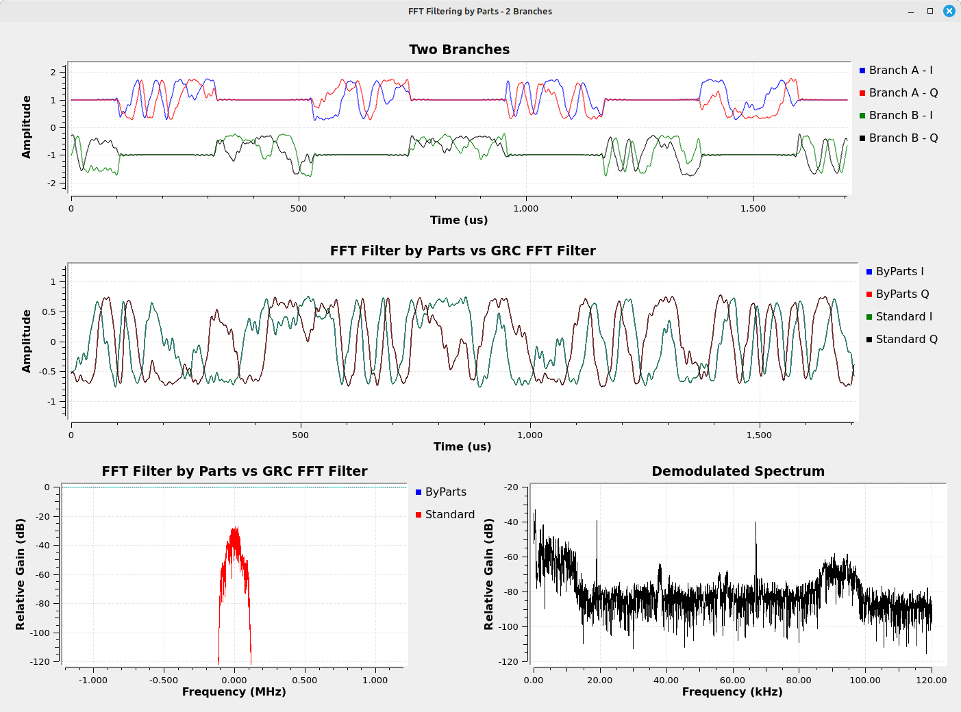
The end result is a continuous, perfectly filtered (or filtered, perfectly continuous) sample stream. Note that this is not exactly how the "FFT Filter" block operates. I'm certain it does not process two streams in parallel. Since it's specifically programmed for GRC, it most likely keeps a running stream which new samples are simply added to before going to the output. (Yes, the grammar of that last sentence sucks. But... whatever.)

Summary

The point of this post was to demonstrate how FFT convolution works. The general flow is:

Calculate the filter taps, zeropad them, then calculate the FFT of these zeropadded taps.
Pull out a certain number of signal samples, depending on how large the FFT will be.
Zeropad the signal samples such that it is the same number of points as the zeropadded filter taps.
Calculate the FFT of the zeropadded signal samples.
Multiply the two FFTs (zeropadded filter taps and zeropadded signal samples) together.
Calculate the inverse FFT to convert back to the time domain.
Add output of inverse FFT to previous output to create continuous stream.
Repeat steps 2 - 7.

A couple of other points:

To repeat, do not window the data before calculating the FFT. Windowing is used when you're performing spectral analysis and you need to get rid of the issues of spectral leakage. When you're performing spectral processing, you don't use any windowing. In GRC, the easy way to do this is to set the window to rectangular (e.g. "window.rectangular(512)"). This is the equivalent of no windowing.
The number of signal samples is totally arbitrary. For example, even though I used 512 samples in my flowgraph above, I could have used 1024 or 2048 while using an equal number of zeros and double the number of points (so a 4096 point FFT for 2048 samples, or 8192 point FFT for 4096 samples). If I was actually programming this, I could set the number of samples to pretty much whatever I want. I could increase the the size to, say, 8192 samples. This would require adding a lot more zeros to the filter taps, but since that calculation only has to be done once, that probably is a net savings and allows the FFT to really provide much more efficiency.

That's it for now. Til next time!

Random Quote Board